Electromagnetic wave propagation

Plane waves are a well-known solution to Maxwell's equations in a non-conducting, source-free, anisotropic linear dielectric medium

\[ \nabla \times \nabla \times {\bf E} = -\mu {\boldsymbol \epsilon} \frac{\partial^2 {\bf E}}{\partial t^2}, \]

where ${\bf E}$ is the electric field, ${\boldsymbol \epsilon}$ is the bulk dielectric permittivity tensor, and $\mu$ the bulk isotropic permeability of the medium. Note this can also be written as $\nabla^2 {\bf E} = \mu {\boldsymbol \epsilon} {\partial^2 {\bf E}}/{\partial t^2}$. Substituting ${\bf E}$ for a plane wave solution, ${\bf E} = {\bf E}_0 \exp[i({\bf k}\cdot {\bf x} - \omega t)]$, the problem reduces to

\[ ({\bf K} + \omega^2 \mu {\boldsymbol \epsilon}) {\bf E} = {\bf 0}, \]

where ${\bf K} = {\bf k}\times{\bf k} \times$ is the matrix representation of the twice-applied cross product. The above equation requires

\[ \det( {\bf K} + \omega^2 \mu {\boldsymbol \epsilon} ) = 0 . \]

Evidently, the eigenvalues and eigenvectors of ${\boldsymbol \epsilon}^{-1} {\bf K}/(\mu k^2)$ are the permitted wave velocities squared and wave polarization, respectively, where

\[ V^2 = \frac{\omega^2}{k^2} \]

is the wave velocity squared.

Homogenization

If wave lengths are much longer than the average grain size, the problem can be closed by approximating the bulk polycrystalline permittivity tensor by the grain-averaged permittivity tensor

\[{\boldsymbol \epsilon} = \langle {\boldsymbol \epsilon}' \rangle,\]

constructed by averaging over all grain orientations (over the CPO).

Glacier ice

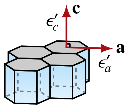
If ice grains are approximated as transversely isotropic w.r.t. the $c$-axis, the dielectric permittivity tensor of a single crystal can be written as $$ {\boldsymbol \epsilon}' = (2\epsilon_{a}' + \epsilon_{c}') \frac{\bf I}{3} + (\epsilon_{c}'-\epsilon_{a}') \left( {\bf c}^2 - \frac{\bf I}{3} \right), $$ where $\epsilon_{c}'$ and $\epsilon_{a}'$ are the permittivities parallel and perpendicular to the $c$ axis. In this case, the grain-averaged permitivity is simply

\[ \langle {\boldsymbol \epsilon}'\rangle = (2\epsilon_{a}' + \epsilon_{c}') \frac{\bf I}{3} + (\epsilon_{c}'-\epsilon_{a}') \left( \langle {\bf c}^2 \rangle - \frac{\bf I}{3} \right) , \]

where $\langle {\bf c}^2 \rangle$ is the second-order structure tensor.

Code example

Experimental, bug reports are welcome.

import numpy as np
from specfabpy import specfab as sf
lm, nlm_len = sf.init(4)
nlm = np.zeros((nlm_len), dtype=np.complex64) # array of expansion coefficients

### Physical parameters (note eps=eps0*epsr, mu=mu0*mur)
epsr_c = 3.17        # relative permittivity of a single grain parallel to symmetry axis (c) 
epsr_a = 3.17-0.034  # relative permittivity of a single grain perpendicular to symmetry axis (a)
mur = 1              # relative permeability of a single grain

### CPO from second-order structure tensor
p = np.array([0,0,1]) # preferred c-axis direction
a2 = np.einsum('i,j', p,p) # a2 if MODF = deltafunc(r-p) 
nlm[:sf.L2len] = sf.a2_to_nlm(a2) # l<=2 expansion coefficients

### Propagation directions of interest
theta, phi = np.deg2rad([0,90,]), np.deg2rad([0,0,]) # theta=colatitude, phi=longitude

### Calculate phase velocities
Vi = sf.Vi_electromagnetic_tranisotropic(nlm, epsr_c, epsr_a, mur, theta,phi) # fast and slow phase velocities are V_S1=vi[0,:], V_S2=vi[1,:]

The below animation shows directional S-wave velocities for a CPO evolving under $xz$ confined compression, relative to an isotropic CPO, when subject to lattice rotation.

Olivine

🚧 Not yet supported.