Elastic wave propagation

Problem

We seek plane wave solutions of the Cauchy-Navier equation of motion

\[ \nabla\cdot {\boldsymbol \sigma} = \rho \frac{\partial^2 {\bf d}}{\partial t^2}, \]

where \({\boldsymbol \sigma}\) is the bulk stress tensor, \({\bf d}\) is the displacement field, and \(\rho\) the mass density.

Substituting \({\bf d}\) for a plane wave solution, \({\bf d} = {\bf d}_0 \exp[i({\bf k}\cdot {\bf x} - \omega t)]\), the problem reduces to

\[ (k^2\hat{{\bf Q}} - \omega^2 \rho {\bf I}) {\bf d} = {\bf 0}, \]

where \(\hat{{\bf Q}}(\hat{{\bf k}})\) is the normalized acoustic tensor that varies depending on the bulk constitutive equation substituted for \({\boldsymbol \sigma}({\bf d})\).

The above equation requires

\[ \det( k^2\hat{{\bf Q}} - \omega^2 \rho {\bf I} ) = 0 . \]

Evidently, the eigenvalues and eigenvectors of \(\hat{{\bf Q}}/\rho\) are the permitted wave velocities squared and wave polarization, respectively, where

\[ V^2 = \frac{\omega^2}{k^2} \]

is the wave velocity squared.

Homogenization

The problem may be closed by approximating \(\hat{{\bf Q}}\) as the grain-averaged acoustic tensor, subject to a linear combination of the Voigt and Reuss homogenization schemes:

\[ \hat{{\bf Q}} = (1-\alpha) \langle\hat{{\bf Q}}'_{\mathrm{Reuss}}\rangle + \alpha \langle \hat{{\bf Q}}'_{\mathrm{Voigt}}\rangle . \]

The Voigt scheme (\(\alpha=1\)) assumes the strain field is homogeneous over the polycrystal scale, whereas the Reuss scheme (\(\alpha=0\)) assumes the stress is homogeneous.

In these homogenizations, grains are therefore assumed interactionless and the bulk elastic behaviour is therefore simply the grain-orientation-averaged elastic behaviour subject to either homogeneous stress or strain assumptions over the polycrystal scale.

Grain parameters

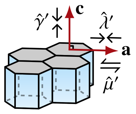
The grain elastic parameters used for homogenization should be understood as the effective polycrystal values needed to reproduce experimental results; they are not the values derived from experiments on single crystals.

Transversely isotropic grains

Monocrystal	Polycrystal

If grains are approximately transversely isotropic, the grain elastic behaviour can be modelled using the transversely isotropic elastic constitutive equation. This requires specifying the grain elastic parameters \(\lambda'\), \(\mu'\), \(\hat{\lambda}'\), \(\hat{\mu}'\), \(\hat{\gamma}'\), and the Voigt—Reuss weight \(\alpha\).

Example for glacier ice

import numpy as np
from specfabpy import specfab as sf
lm, nlm_len = sf.init(4) # L=4 is sufficient here
nlm = np.zeros((nlm_len), dtype=np.complex64) # array of expansion coefficients

### c-axis number distribution (nlm) from fourth-order structure tensor (a4)
p = np.array([0,0,1]) # preferred c-axis direction
a4 = np.einsum('i,j,k,l', p,p,p,p) # a4 if ODF = deltafunc(r-p) 
nlm[:sf.L4len] = sf.a4_to_nlm(a4) # determine l<=4 expansion coefficients of ODF

### Physical parameters (SI units)
rho = 917 # density of ice
Cij = (14.060e9, 15.240e9, 3.060e9, 7.150e9, 5.880e9) # Bennett (1968) parameters (C11,C33,C55,C12,C13)
Lame_grain = sf.Cij_to_Lame_tranisotropic(Cij) # Lame parameters (lam,mu,Elam,Emu,Egam)
alpha = 0.5 # Voigt--Reuss weight, where 0.5 = Hill average

### Propagation directions of interest
theta, phi = np.deg2rad([90,70,]), np.deg2rad([0,10,]) # wave-vector directions (theta is colatitude, phi is longitude)

### Calculate phase velocities
Vi = sf.Vi_elastic_tranisotropic(nlm, alpha, Lame_grain, rho, theta,phi) # phase velocities are V_S1=vi[0,:], V_S2=vi[1,:], V_P=vi[2,:]

Evolving CPO

The below animation shows directional P- and S-wave velocities for a CPO evolving under uniaxial compression along \({\hat {\bf z}}\), relative to an isotropic CPO, when subject to lattice rotation.

Orthotropic grains

Monocrystal	Polycrystal

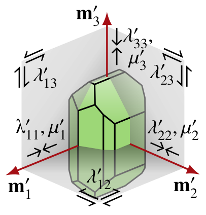
If grains are approximately orthotropic, the grain elastic behaviour can be modelled using the orthotropic elastic constitutive equation. This requires specifying the grain elastic parameters \(\lambda_{ij}'\), \(\mu_{i}'\), and the Voigt—Reuss weight \(\alpha\).

Example for olivine

import numpy as np
from specfabpy import specfab as sf
lm, nlm_len = sf.init(4) # L=4 is sufficient here
nlm = np.zeros((nlm_len), dtype=np.complex64) 
blm = np.zeros((nlm_len), dtype=np.complex64) 

### Grain orientation distributions (nlm,blm) from fourth-order structure tensors
vn = np.array([0,0,1]) # preferred slip-normal direction
vb = np.array([1,0,0]) # preferred slip direction
a4_n = np.einsum('i,j,k,l', vn,vn,vn,vn) # a4 if n/N ODF = deltafunc(r-vn) 
a4_b = np.einsum('i,j,k,l', vb,vb,vb,vb) # a4 if b/N ODF = deltafunc(r-vb) 
nlm[:sf.L4len] = sf.a4_to_nlm(a4_n) # determine l<=4 expansion coefficients of ODF
blm[:sf.L4len] = sf.a4_to_nlm(a4_b) # determine l<=4 expansion coefficients of ODF

### Physical parameters (SI units)
rho = 3355 # density of olivine
alpha = 1 # Voigt--Reuss weight; only alpha=1 supported for now
Cij = (320.5e9, 196.5e9, 233.5e9,  64.0e9, 77.0e9, 78.7e9,  76.8e9, 71.6e9, 68.15e9) # Abramson (1997) parameters (C11,C22,C33,C44,C55,C66,C23,C13,C12)
Lame_grain = sf.Cij_to_Lame_orthotropic(Cij) # Lame parameters (lam11,lam22,lam33, lam23,lam13,lam12, mu1,mu2,mu3)
# Note that the above ordering of Lame/Cij parameters assume an A-type fabric; that is, (blm,nlm,vlm) refer to the distibutions of (m1',m2',m3') axes, respectively.
# If concerned with another fabric type, the components can easily be re-ordered:
#Lame_grain = sf.Lame_olivine_A2X(Lame_grain, 'B') # B-type Lame paremeters
#Lame_grain = sf.Lame_olivine_A2X(Lame_grain, 'C') # C-type Lame paremeters

### Propagation directions of interest
theta, phi = np.deg2rad([90,70,]), np.deg2rad([0,10,]) # wave-vector directions (theta is colatitude, phi is longitude)

### Calculate phase velocities
vlm = 0*nlm # estimate vlm from (blm,nlm) by passing zero array
Vi = sf.Vi_elastic_orthotropic(blm,nlm,vlm, alpha, Lame_grain, rho, theta,phi) # phase velocities are V_S1=vi[0,:], V_S2=vi[1,:], V_P=vi[2,:]