Lattice rotation
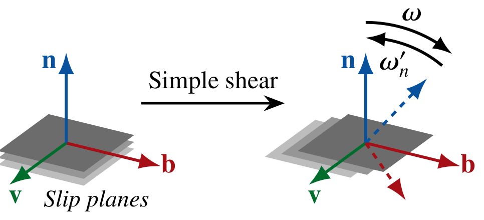
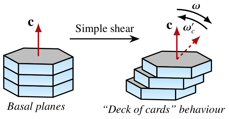
When subject to simple shear, the orientation of easy slip systems in polycrystalline materials like ice or olivine tend towards aligning with the bulk shear-plane system. That is, the \(n\)-axis (\(c\)-axis in ice) tends towards to bulk shear plane normal, and the \(b\)-axis (\(a\)-axis in ice) towards to bulk shear direction. Thus, if grains are perfectly aligned with the bulk shear system, their orientation should be unaffected by any further shearing, but be in steady state. Clearly, slip systems do therefore not simply co-rotate with the bulk continuum spin (\({\boldsymbol \omega}\)) like passive material line elements embedded in a flow field, i.e. \({\bf \dot{n}} \neq {\boldsymbol \omega} \cdot {\bf n}\). Rather, slip systems must be subject to an additional contribution — a plastic spin \({\boldsymbol\omega}'\) — such that the bulk spin is exactly counteracted to achieve steady state if favorably aligned:
More precisely, the crystallographic axes reorient themselves in response to both the bulk continuum spin and a plastic spin that is supposed to represent the crystallographic spin needed to accommodate strain compatibility between grains that otherwise preferentially deform by easy slip (i.e., basal slip for ice).
Directors method
Aravas and Aifantis (1991) and Aravas (1994) (among others) proposed a particularly simple model for the functional form of \({\boldsymbol \omega}'\), the so-called directors method.
For a constant rate of shear deformation (\(1/\tau\)) aligned with the \({\bf b}\)—\({\bf n}\) system, the deformation gradient is \({\bf F} = {\bf I} + (t/\tau) {\bf b}{\bf n}\) and therefore
Since \({\boldsymbol \omega}' = -{\boldsymbol \omega}\) is required in steady state, it follows from eliminating \(1/(2\tau)\) by calculating \({\dot{\boldsymbol\epsilon}} \cdot {\bf n}^2\), \({\bf n}^2 \cdot {\dot{\boldsymbol\epsilon}}\), \({\dot{\boldsymbol\epsilon}} \cdot {\bf b}^2\), and \({\bf b}^2 \cdot {\dot{\boldsymbol\epsilon}}\), that
Indeed, this result agrees with representation theorems for isotropic functions (Wang, 1969), stating that an antisymmetric tensor-valued function of a symmetric tensor (\({\dot{\boldsymbol\epsilon}}\)) and a vector (\({\hat {\bf r}}\)) is to lowest order given by
To be consistent with the above, \(\iota = +1\) for \({\hat {\bf r}}={\bf n}\) and \(\iota = -1\) for \({\hat {\bf r}}={\bf b}\).
\({\boldsymbol \omega}'_{n}\) and \({\boldsymbol \omega}'_{b}\) are then generally taken to suffice for other deformation kinematics, too.
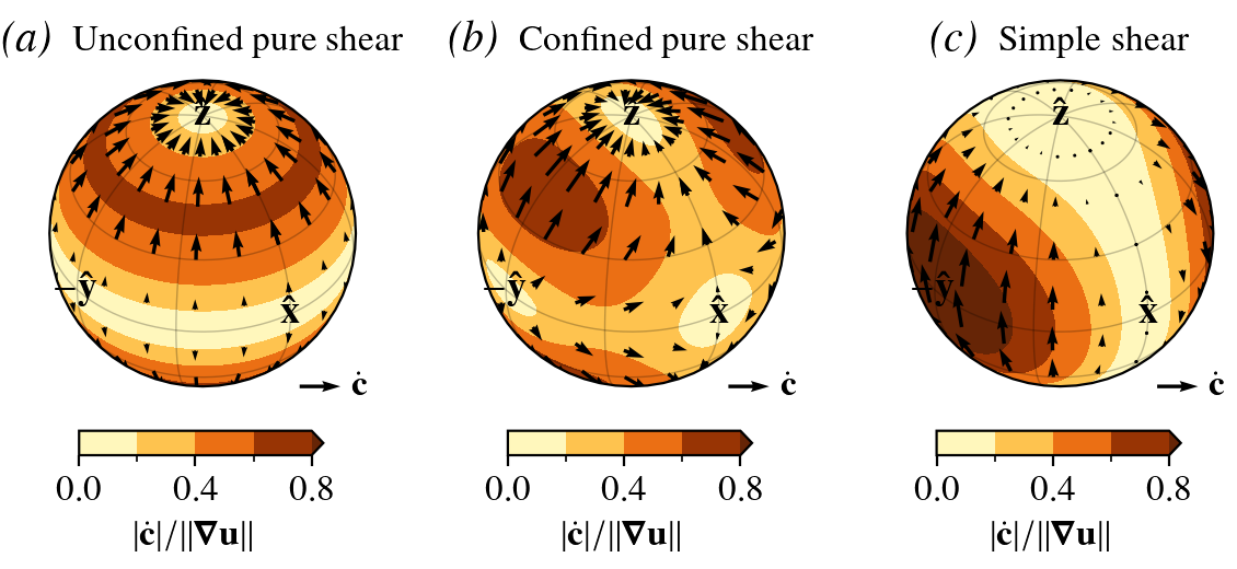
Glacier ice
The predicted normalized \(c\)-axis velocity field for glacier ice where \({\bf n} = {\bf c}\) is show below for three different deformation kinematics:

Matrix model
The corresponding effect on the continuous distribution functions is modelled as a conservative advection process in orientation space \(S^2\):
where \({\bf M_{\mathrm{LROT}}}(\iota)\) is given analytically in Rathmann et al. (2021).
Code example
import numpy as np
from specfabpy import specfab as sf
# L=8 truncation is sufficient in this case, but larger L allows a very strong fabric to
#  develop and minimizes the effect that regularization has on low wavenumber modes (l=2,4)
lm, nlm_len = sf.init(8)

### Velocity gradient tensor experienced by parcel

ugrad = np.diag([0.5, 0.5, -1.0]) # uniaxial compression along z-axis
D = (ugrad+np.transpose(ugrad))/2 # symmetric part (strain rate tensor)
W = (ugrad-np.transpose(ugrad))/2 # anti-symmetric part (spin tensor)

### Numerics

Nt = 25   # number of time steps
dt = 0.05 # time-step size

### Initial fabric state

nlm = np.zeros((Nt,nlm_len), dtype=np.complex64) # n state vector
nlm[0,0] = 1/np.sqrt(4*np.pi) # normalized isotropic state at t=0

### Euler integration

for tt in np.arange(1,Nt):
    nlm_prev = nlm[tt-1,:] # previous solution
    iota, zeta = 1, 0      # "deck of cards" behavior
    M_LROT = sf.M_LROT(nlm_prev, D, W, iota, zeta) # lattice rotation operator
    M_REG  = sf.M_REG(nlm_prev, D)                 # regularization operator
    M      = M_LROT + M_REG
    nlm[tt,:] = nlm_prev + dt*np.matmul(M, nlm_prev) # euler step
    nlm[tt,:] = sf.apply_bounds(nlm[tt,:]) # apply spectral bounds if needed