Lagrangian CPO parcel

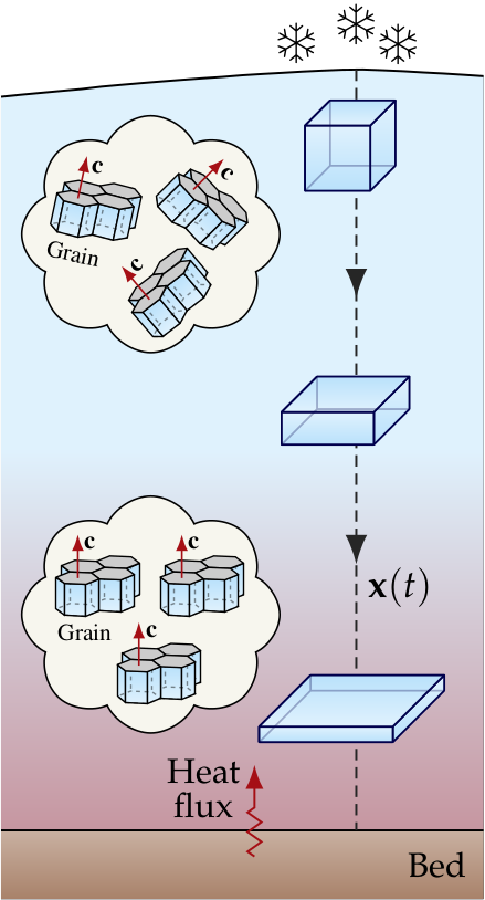
A Lagrangian parcel refers to a small, moving material volume that is followed through time as it flows within e.g. a glacier or ice sheet, unlike the Eulerian perspective which focuses on fixed locations in space. A Lagrangian description is well-suited for studying CPO evolution along a flow line \({\bf x}(t)\) if the thermomechanical background conditions are approximately steady; that is, the velocity, temperature, and stress fields are constant in time, though not necessarily in space. By treating each parcel as a discrete entity with its own microstructural state that updates with time, a Lagrangian parcel model is a particularly simply way to estimate CPO evolution and to calculate CPO-induced quantities along a flow line (trajectory), such as mechanical or dielectric anisotropy.
Below, some examples are given on how to model CPO evolution using the Lagrangian parcel approach, relevant to glacier ice.
Ice divide
A Lagrangian approach is well-suited for modelling the vertical CPO profile at domes and divides of ice sheets. Assuming e.g. the classical Nye model of an ice divide of height \(H\) (no basal melt, constant rate of thinning, a constant accumulation rate \(a\)), the velocity gradient is constant and equal to
where \(q=0\) for a axis-symmetric dome and \(q=\pm 1\) for a divide aligned with the \(x\) or \(y\) direction. The \(e\)-folding time \(\tau\) is a function of the ice-equivalent accumulation rate and divide thickness:
Depending on whether temperatures are large enough to activate DDRX or not, the temperature profile must be prescribed, too.
📝 Example: GRIP ice core
The following code example shows how to model the CPO profile of the GRIP ice core, Greenland. Eigenvalues of other ice cores can be found here.
The figure to the right shows the model result (lines) compared to observations (markers) from thin-section analysis. At around \(z/H \simeq 0.2\), temperatures are sufficiently high that DDRX becomes important and affects (weakens) the vertical single-maximum CPO that otherwise strengthens with depth.

"""
Model CPO profile of the GRIP ice core, Greenland
"""

import numpy as np
from scipy.integrate import solve_ivp
from scipy import interpolate
import pandas as pd

from specfabpy import specfab as sf
from specfabpy import common as sfcom
from specfabpy import plotting as sfplt

import matplotlib.pyplot as plt

from matplotlib import rc
#rc('font',**{'family':'sans-serif','sans-serif':['Helvetica']})
rc('font',**{'family':'serif','serif':['Palatino']})
rc('text', usetex=True)

"""
Setup
"""

### Velocity gradient experienced by parcel

H   = 3027 # ice thickness (Montagnat et al., 2014)
a   = 0.24 # meter ice equiv. per yr (Montagnat et al., 2014)
tau = H/a  # e-folding time scale
ugrad = -1/tau*np.diag([-0.5, -0.5, 1]) # uniaxial compression along z-axis

### Numerics

tend = 50e3 # time (in years) to trace out trajectory, starting from the surface
#tend = -tau*np.log(0.05) # alternatively, set tend so that simulation stops at 95% thinning

Nt = 1000 # number of time steps taken (increase this until results are robust)
ti = np.linspace(0, tend, Nt) # time points at which to evaluate the solution
z  = np.exp(-ti/tau) # relative height above bed at each point in time

L = 12 # CPO expansion series truncation
kw_ivp = dict(method='RK45', vectorized=False) # kwargs for solve_ivp()

### CPO dynamics

# Lattice rotation
iota, zeta = 1, 0 # "deck of cards" behavior

# DDRX
A = 1.1e7  # rate prefactor (tunable parameter)
Q = 3.36e4 # activation energy (see Richards et al. (2021) and Lilien et al. (2023))
R = 8.314  # gas constant
Gamma0 = lambda D, T: A*np.sqrt(np.einsum('ij,ji',D,D)/2)*np.exp(-Q/(R*(T+273.15))) # DDRX rate factor

### Temperature profile

df = pd.read_csv('../../../data/icecores/GRIP/temperature.csv') # fetch from github
fz = interpolate.interp1d(df['zrel'].to_numpy(), df['T'].to_numpy(), kind='linear', fill_value='extrapolate')
T = fz(z) # temperature profile

"""
Solve CPO evolution
"""

D = (ugrad+np.transpose(ugrad))/2 # symmetric part (strain rate tensor)
W = (ugrad-np.transpose(ugrad))/2 # anti-symmetric part (spin tensor)
S = D # stress tensor (assume coaxiality with strain-rate tensor; magnitude does not matter for our purpose)

#T[:] = -60 # no DDRX if ice is very cold

lm, nlm_len = sf.init(L) # initialize specfab
lh_init = 0.25 # initial horizontal eigenvalues
a2_init = np.diag([lh_init, lh_init, 1-2*lh_init]) # initial a2 (at surface)

nlm_init = np.zeros((nlm_len), dtype=np.complex64) # CPO expansion coefficients
nlm_init[:sf.L2len] = sf.a2_to_nlm(a2_init) # initial state vector (at surface)

def ODE(t, nlm):
    # d/dt nlm_i = M_ij . nlm_j, where nlm_i is the state vector (aka s_i)
    I = np.argmin(np.abs(ti-t)) # index for closest point on trajectory at time t
    M  = sf.M_LROT(nlm, D, W, iota, zeta) # lattice rotation always present
    M += Gamma0(D,T[I])*sf.M_DDRX(nlm, S) # DDRX active if sufficient warm
    #M += Lambda0*sf.M_CDRX(nlm)          # CDRX (neglected in this example)
    M += sf.M_REG(nlm, D)                 # regularization
    return np.matmul(M, nlm)

nlm = solve_ivp(ODE, (0, tend), nlm_init, t_eval=ti, vectorized=False).y.T # CPO state along trajectory
mi, lami = sfcom.eigenframe(nlm) # a2 eigenvectors and eigenvalues

"""
Plot results
"""

### Plot modeled eigenvalues

fig = plt.figure(figsize=(3,4))
ax = plt.subplot(111)

c1,c2,c3 = 'tab:blue', 'tab:red', 'k'

ax.plot(lami[:,0], z, '-',  c=c1, label=r'$\lambda_1$')
ax.plot(lami[:,1], z, '-',  c=c2, label=r'$\lambda_2$')
ax.plot(lami[:,2], z, '--', c=c3, label=r'$\lambda_3$')

ax.legend(loc=1, fancybox=False, frameon=False)
ax.set_title(r'GRIP ice core')

ax.set_xlabel(r'$\lambda_i$')
ax.set_xticks(np.arange(0,1+.01,0.2))
ax.set_xlim([0,1])

ax.set_ylabel(r'$z/H$')
ax.set_yticks(np.arange(0,1+.01,0.1))
ax.set_ylim([0,1])

### Plot CPOs

geo, prj = sfplt.getprojection(rotation=45, inclination=50)

def plotCPO(ax, nlm, p0, HW=0.2, cmap='Greys'):
    axtrans = ax.transData.transform(p0)
    trans = fig.transFigure.inverted().transform(axtrans)
    axin = plt.axes([trans[0]-HW/2, trans[1]-HW/2, HW,HW], projection=prj)
    axin.set_global()
    lvlset = [np.linspace(0.05, 0.45, 8), lambda x,p:'%.1f'%x]
    sfplt.plotODF(nlm, lm, axin, lvlset=lvlset, cmap=cmap, showcb=False, nchunk=None)
    sfplt.plotcoordaxes(axin, geo, negaxes=False, color=sfplt.c_dred, axislabels='xi')
    return axin

for zi in np.linspace(0.1, 0.9, 4):
    I = np.argmin(np.abs(z-zi))
    plotCPO(ax, nlm[I], (1.2,zi))

### Plot observations

df = pd.read_csv('../../../data/icecores/GRIP/orientations.csv') # fetch from github
zobs = df['zrel'].to_numpy()
kw = dict(marker='o', facecolor='none', zorder=1)
ax.scatter(df['lam1'].to_numpy(), zobs, edgecolor=c1, **kw)
ax.scatter(df['lam2'].to_numpy(), zobs, edgecolor=c2, **kw)
ax.scatter(df['lam3'].to_numpy(), zobs, edgecolor=c3, **kw)

### Save plot

plt.savefig('GRIP-parcel.png', dpi=175, pad_inches=0.1, bbox_inches='tight')
Plug flow

If the Shallow Shelf/Stream Approximation (SSA) is applicable, velocities can be assumed depth constant (i.e., plug flow without vertical shearing). In this case, a depth-average treatment of CPO evolution transforms the Lagrangian parcel model into a Lagrangian column model. This generalizes the above parcel model, since the velocity gradient and stress fields can no longer be assumed constant but depend on the column position \({\bf x}(t)=[x(t),y(t)]\).
Assuming that both velocity and CPO fields are steady, and neglecting surface accumulation that adds new (isotropic) ice, the problem can be solved by prescribing satellite-derived surface velocities and estimates of the ice temperature.
📝 Example: Pine Island Glacier
The following code example shows how to model CPO evolution along a flow line over the Pine Island Glacier, Antarctica. The example relies on MEaSUREs ice velocities, assumes a constant temperature field, and asserts that the stress tensor can be approximated as coaxial to the strain rate tensor to close the DDRX problem. If the ice mass is sufficiently cold, DDRX can be neglected altogether and only satellite-derived velocities are needed to close the problem.

"""
Model plug-flow CPO evolution of a Lagrangian ice column over Pine Island Glacier, Antarctica
"""

import numpy as np
from scipy.integrate import solve_ivp
import xarray

from specfabpy import specfab as sf
from specfabpy import common as sfcom
from specfabpy import plotting as sfplt

import matplotlib.pyplot as plt
from mpl_toolkits.axes_grid1 import make_axes_locatable
import matplotlib.colors as colors

from matplotlib import rc
#rc('font',**{'family':'sans-serif','sans-serif':['Helvetica']})
rc('font',**{'family':'serif','serif':['Palatino']})
rc('text', usetex=True)

"""
Setup
"""

### Domain

p0   = (-1500e3, -70e3)  # starting point (x0,y0)
xy0  = (-1710e3, -335e3) # lower left-hand  corner of region of interest
xy1  = (-1425e3, -50e3)  # upper right-hand corner of region of interest
dwin = 2 # coarsen input velocities using this moving-average window size

tend = 820 # time (in years) to trace out trajectory from staring point

### Numerics

Nt = 1000 # number of time steps taken (increase this until results are robust)
L = 12 # CPO expansion series truncation
kw_ivp = dict(method='RK45', vectorized=False) # kwargs for solve_ivp()

### CPO dynamics

# Lattice rotation
iota, zeta = 1, 0 # "deck of cards" behavior

# DDRX
A = 1.1e7  # rate prefactor (tunable parameter)
Q = 3.36e4 # activation energy (see Richards et al. (2021) and Lilien et al. (2023))
R = 8.314  # gas constant
Gamma0 = lambda D, T: A*np.sqrt(np.einsum('ij,ji',D,D)/2)*np.exp(-Q/(R*(T+273.15))) # DDRX rate factor

"""
Determine trajectory
"""

### Velocity field

print('*** Loading velocity field')

ds0 = xarray.open_mfdataset('~/ice-velocity-maps/antarctica_ice_velocity_450m_v2.nc') # MEaSUREs
uxname, uyname = 'VX', 'VY'
xr = slice(xy0[0], xy1[0])
yr = slice(xy1[1], xy0[1]) # reverse on purpose
ds = ds0.sel(x=xr,y=yr).coarsen(x=dwin, boundary='trim').mean().coarsen(y=dwin, boundary='trim').mean()

### Determine trajectory

print('*** Determining trajectory')

def ODE_traj(t, p):
    dsi = ds.interp(x=p[0], y=p[1], method='linear')
    return [dsi[uxname].to_numpy(), dsi[uyname].to_numpy()] # [ux, uy]

trng = (0, tend)
ti = np.linspace(trng[0], trng[1], Nt) # time points at which to evaluate the solution
pi = solve_ivp(ODE_traj, trng, p0, t_eval=ti, vectorized=False).y # trajectory [x(t), y(t)]

### Determine velocity gradient tensor along trajectory

print('*** Determining velocity gradients')

ds_grad = xarray.Dataset({
    'duxx': ds[uxname].differentiate('x'),
    'duxy': ds[uxname].differentiate('y'),
    'duyx': ds[uyname].differentiate('x'),
    'duyy': ds[uyname].differentiate('y'),
})
ds_gradi = ds_grad.interp(x=('points', pi[0]), y=('points', pi[1]), method='linear')

ugrad = np.zeros((Nt,3,3))
ugrad[:,0,0] = ds_gradi['duxx'].values
ugrad[:,0,1] = ds_gradi['duxy'].values
ugrad[:,1,0] = ds_gradi['duyx'].values
ugrad[:,1,1] = ds_gradi['duyy'].values
ugrad[:,2,2] = -(ugrad[:,0,0]+ugrad[:,1,1]) # incompressible ice

D = (ugrad + np.einsum('ijk->ikj',ugrad))/2 # strain rate tensor
W = (ugrad - np.einsum('ijk->ikj',ugrad))/2 # stress tensor

"""
Solve CPO evolution
"""

print('*** Solving CPO evolution')

S = D # stress tensor (assume coaxiality with strain-rate tensor; magnitude does not matter for our purpose)

#T = -30 # temperature assumed constant along flow line (deg. C)
T = -60 # no DDRX if ice is very cold

# isotropic initial state
lm, nlm_len = sf.init(L) # initialize specfab
nlm_init = np.zeros((nlm_len), dtype=np.complex64) # CPO expansion coefficients
nlm_init[0] = 1/np.sqrt(4*np.pi)

def ODE(t, nlm):
    # d/dt nlm_i = M_ij . nlm_j, where nlm_i is the state vector (aka s_i)
    I = np.argmin(np.abs(ti-t)) # index for closest point on trajectory at time t
    M  = sf.M_LROT(nlm, D[I], W[I], iota, zeta) # lattice rotation always present
    M += Gamma0(D[I],T)*sf.M_DDRX(nlm, S[I])    # DDRX active if sufficient warm
    #M += Lambda0*sf.M_CDRX(nlm)                # CDRX (neglected in this example)
    M += sf.M_REG(nlm, D[I])                    # regularization
    return np.matmul(M, nlm)

nlm = solve_ivp(ODE, trng, nlm_init, t_eval=ti, vectorized=False).y.T # CPO state along trajectory
mi, lami = sfcom.eigenframe(nlm) # a2 eigenvectors and eigenvalues

"""
Plot results
"""

print('*** Plotting results')

fs  = 1.0 # figure scale
fig = plt.figure(figsize=(9*fs,2.5*fs))
gs  = fig.add_gridspec(nrows=1, ncols=2, wspace=0.20)
ax1, ax2 = fig.add_subplot(gs[0,0]), fig.add_subplot(gs[0,1])

ms = 1e-3 # mapscale (m to km)
c1,c2,c3 = 'tab:blue', 'tab:red', 'k'
ctraj = 'limegreen'

### Plot trajectory over velocity map

# Create regular grid for plotting velocity field
N = 200
xv = np.linspace(xy0[0], xy1[0], N)
yv = np.linspace(xy0[1], xy1[1], N)
X, Y = np.meshgrid(xv, yv)
dsi = ds.interp(x=xv, y=yv, method='linear') # interpolate ux and uy to new grid
UX, UY = dsi[uxname].to_numpy(), dsi[uyname].to_numpy()
U = np.sqrt(np.power(UX,2) + np.power(UY,2))

# Plot velocity map
lvls = np.logspace(0.5, 3.75, 14)
norm = colors.LogNorm(vmin=lvls[0], vmax=lvls[-1])
cs = ax1.contourf(X*ms, Y*ms, U, cmap='inferno', levels=lvls, norm=norm, extend='both')
cax = make_axes_locatable(ax1).append_axes('right', size="5%", pad=0.08)
plt.colorbar(cs, label=r'$u$ (m/yr)', cax=cax)
ax1.streamplot(X[0]*ms, Y[:,0]*ms, UX, UY, color='0.7', linewidth=0.4, density=0.8)
ax1.plot(pi[0]*ms, pi[1]*ms, '-', c=ctraj, lw=2)
ax1.plot(p0[0]*ms, p0[1]*ms, 'o', c=ctraj, markeredgewidth=2, markerfacecolor='none', markersize=10)

ax1.axis('square')
ax1.set_xlim([xy0[0]*ms, xy1[0]*ms])
ax1.set_ylim([xy0[1]*ms, xy1[1]*ms])
ax1.set_xlabel('$x$ (km)')
ax1.set_ylabel('$y$ (km)')
ax1.set_title(r'Pine Island Glacier')

### Plot eigenvalues

dl = np.sqrt(np.diff(pi[0])**2 + np.diff(pi[1])**2) # segment lengths of trajectory
l = np.concatenate([[0], np.cumsum(dl)]) # cumulative sum (distance along trajectory)

ax2.plot(l*ms, lami[:,0], c=c1, label=r'$\lambda_1$')
ax2.plot(l*ms, lami[:,1], c=c2, label=r'$\lambda_2$')
ax2.plot(l*ms, lami[:,2], c=c3, label=r'$\lambda_3$')
ax2.legend(loc='center right', fancybox=False, frameon=False)

ax2.set_ylabel(r'$\lambda_i$')
ax2.set_ylim([0,1])
ax2.set_xlabel('Distance along flow line (km)')
ax2.set_xlim([l[0]*ms,l[-1]*ms])

### Plot CPOs

# Make space for CPOs above eigenvalue plot
ax3 = make_axes_locatable(ax2).append_axes("top", size="35%", pad=0.00)
ax3.set_axis_off()

geo, prj = sfplt.getprojection(rotation=-45, inclination=50)

def plotCPO(ax, nlm, mi, p0, HW=0.23, cmap='Greys'):
    axtrans = ax.transData.transform(p0)
    trans = fig.transFigure.inverted().transform(axtrans)
    axin = plt.axes([trans[0]-HW/2, trans[1]-HW/2, HW,HW], projection=prj)
    axin.set_global()
    lvlset = [np.linspace(0.05, 0.45, 8), lambda x,p:'%.1f'%x]
    sfplt.plotODF(nlm, lm, axin, lvlset=lvlset, cmap=cmap, showcb=False, nchunk=None)
    sfplt.plotcoordaxes(axin, geo, negaxes=True, color=sfplt.c_dred, axislabels='xi')
    sfplt.plotmi(axin, mi, geo, colors=('gold',), ms=6) # eigenvectors
    return axin

# Plot CPO at selected positions along flow line
for li in np.linspace(l[-1]*0.05, l[-1]*0.9, 4):
    I = np.argmin(np.abs(l-li))
    plotCPO(ax2, nlm[I], mi[I], (li*ms,0.93))

### Save plot

plt.savefig('PIG-column.png', dpi=175, pad_inches=0.1, bbox_inches='tight')