Eulerian CPO field

If the velocity field \({\bf u}({\bf{x}},t)\) and CPO field \({\bf s}({\bf{x}},t)\) can be assumed steady, CPO evolution reduces to a high-dimensional boundary value problem in \({\bf s}({\bf{x}},t)\) that can easily be solved using e.g. the finite element method.

When considering the flow glacier ice, it is common to simplify the problem by invoking the Shallow Shelf Approximation (SSA), a depth-integrated version of the full Stokes equations. This approximation conveniently reduces the problem to a two-dimensional horizontal, membrane-like flow with negligible vertical shear.

Performing a similar calculation, the depth-average expression for steady CPO evolution takes the form (Rathmann et al., 2025)

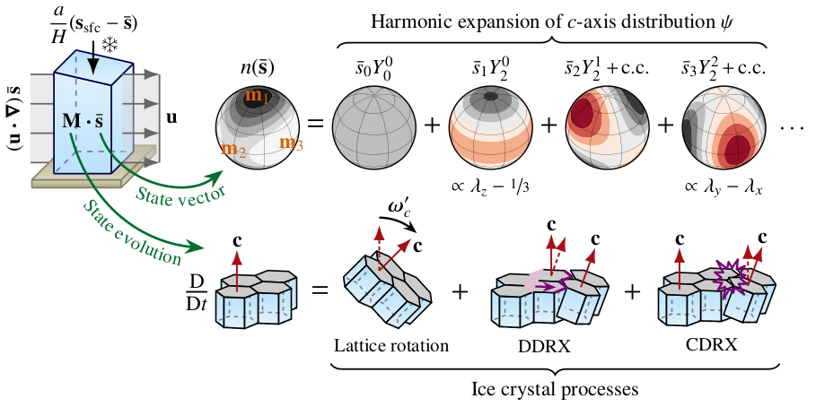
\[ ({\bf u} \cdot \nabla) {\bf \bar s} = ({\bf M}_{\mathrm{LROT}}+{\bf M}_{\mathrm{DDRX}}+{\bf M}_{\mathrm{CDRX}}) \cdot {\bf \bar s} + \frac{a_{\mathrm{sfc}}}{H}( {\bf s}_{\mathrm{sfc}} - {\bf \bar s} ) + \frac{a_{\mathrm{sub}}}{H}( {\bf s}_{\mathrm{sub}} - {\bf \bar s} ) , \]

where \({\bf \bar s}(x,y)\) is the depth-average CPO state vector field, \({\bf{u}}(x,y)=[u_x(x,y),u_y(x,y)]\) is the horizontal surface velocity field, and \(H\) is the ice thickness. The first term represents CPO advection along stream lines, and the second term represents the depth-average effect of crystal processes. The third and fourth terms are state-space attractors, causing \({\bf \bar s}\) to tend towards the characteristic CPO states of ice that accumulates on the surface \({\bf s}_{\mathrm{sfc}}\) or subglacially \({\bf s}_{\mathrm{sub}}\), depending on the positively-defined ice-equivalent accumulation rates \(a_{\mathrm{sfc}}\) and \(a_{\mathrm{sub}}\).

Closure

If CPO development is dominated by lattice rotation (typical for cold ice), the problem is closed by specifying the horizontal surface velocity field (e.g., satellite-derived velocities), together with accumulation rates and the characteristic CPO state of accumulated ice (typically isotropic).

If DDRX is non-negligible (typical for warm ice), the temperature and stress field must additionally be prescribed. In this case, the problem can be closed by assuming some temperature field and assert that the stress and strain-rate tensors are coaxial so that \({\boldsymbol\tau} \propto \dot{\boldsymbol\epsilon}\), although this has some limitations (Rathmann et al., 2025).

Regularization

Noise in surface velocity products, in addition to uncertainties due to model assumptions, can render the steady SSA CPO problem ill-posed. To solve this, Laplacian regularization of the form \(\nu \nabla^2 {\bf \bar s}\) can be adding to the right-hand side of the problem, at the expense of limiting how large spatial CPO gradients are permitted. The strength of regularization \(\nu\) (nu_real in code below) is therefore a free model parameter which must be carefully selected, especially in very dynamic regions where the CPO field might change rapidly with distance.

📝 Example: Pine Island Glacier

Let us consider the Pine Island Glacier (PIG), Antarctica, as an example for how to solve the steady SSA CPO problem, assuming that:

SSA is appropriate for both floating and grounded ice over the region.
CPO development is dominated by englacial crystal processes so that contributions from accumulation can be neglected.
Ice temperatures can be approximated as constant over the domain (needed only if modeling DDRX).

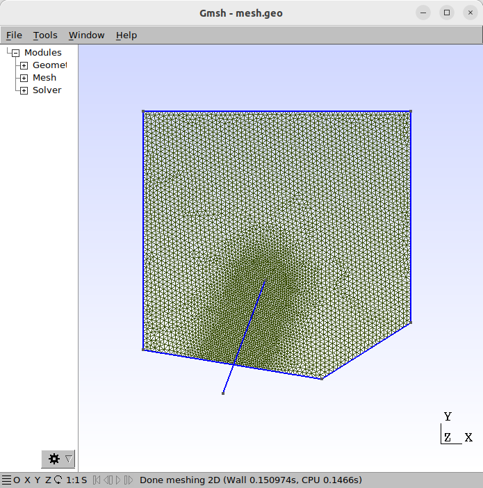
➡️ To begin, the model domain needs to be meshed. For this, we use gmsh with the mesh.geo file:

// *** Mesh of Pine Island Glacier, Antarctica, for steady state SSA CPO solver ***
// Lines 3 to 6 below *must* be the bounding box coordinates of the model domain (to be read by python code)
x0=-1710e3;
y0=-335e3;
x1=-1425e3;
y1=-50e3;

// Mesh resolution
lc=5e3;
lc2=lc/2;

// Mesh corners
Point(1)={x0,-304e3, 0.0,lc};
Point(2)={x0,y1, 0.0,lc};
Point(3)={x1,y1, 0.0,lc};
Point(4)={x1,-275e3, 0.0,lc};
Point(5)={-1520e3,y0, 0.0,lc};

// Connect corners
Line(1)={1,2};
Line(2)={2,3};
Line(3)={3,4};
Line(4)={4,5};
Line(5)={5,1};
Line Loop(5)={1,2,3,4,5};

// Physical lines, etc.
Physical Line(1)={1,2,3,4}; // isotropic boundary on grounded ice
Physical Line(2)={5};       // free boundary on shelf edge
Plane Surface(10)={5};
Physical Surface(11)={10};

// Refine mesh in the neighborhood of a line that passes through trunk of flow
Point(1001)={-1625e3,-350e3,0,lc};
Point(1002)={-1580e3,-230e3,0,lc};
Line(50)={1001,1002};
Field[1]=Distance;
Field[1].CurvesList={50};
Field[2]=Threshold;
Field[2].InField=1;
Field[2].SizeMin=lc2;
Field[2].SizeMax=lc;
Field[2].DistMin=30e3;
Field[2].DistMax=70e3;
Background Field=2;
Mesh.CharacteristicLengthExtendFromBoundary=0; // Don't extend the elements sizes from the boundary inside the domain

which looks like this:

➡️ Next, the CPO problem is solved using FEniCS+specfab and results plotted as follows:

"""
Example of steady state SSA fabric (CPO) solver for Pine Island Glacier, Antarctica
"""

import numpy as np
from specfabpy.fenics.steadyCPO import steadyCPO

SOLVE = True # Solve problem (True) or only plot results (False)?

"""
Model domain
"""

domain = dict(
    name        = 'PIG', # All output file names be prepended by this domain name
    fmeasures   = '~/ice-velocity-maps/antarctica_ice_velocity_450m_v2.nc', # MEaSUREs ice velocities
    fbedmachine = '~/ice-velocity-maps/BedMachineAntarctica-v3.nc',         # BedMachine
    fgeo        = 'mesh.geo', # Gmsh finite element mesh
    subsample_u = 2, # Coarsen input velocities using a moving average with window size "subsample_u" (i.e., no subsampling unless > 1)
    subsample_h = 2, # ...same but for ice thicknesses
)

scpo = steadyCPO(domain)

### Generate mesh and interpolate ice velocities and ice geometry onto mesh
if SOLVE: scpo.preprocess()

"""
Steady CPO problem
"""

problem = dict(
    ### Solve for: lattice rotation + advection
    # - If lattice rotation is dominant then set the temperature to T=None (negligible DDRX; cold ice limit)
    name = 'LROT', 
    T    = None, 

    ### Solve for: lattice rotation + DDRX + advection
    # - If DDRX cannot be neglected, the rate of DDRX is calculated provided the ice temperature and strain rate fields
    # - The rate of DDRX is parameterized using the lab-calibrated temperature activation function of Lilien et al. (2023) (can be changed)
    # - The temperature field T is assumed constant (can be changed)
    # - The solver works by gradually approaching the nonlinear LROT+DDRX solution by starting out assuming no DDRX, then 
    #   gradually increasing the temperature in discrete steps until reaching the desired temperature 
#    name = 'LROT+DDRX', 
#    T    = np.linspace(-40, -15, 4), # Steps of increasing temperatures used to converge on solution for -15C

    ### Boundary conditions (BCs)
    # - BCs are given as a list of mesh "Physical Line" IDs (see mesh.geo) and the CPO state to be imposed there
    # - Two different CPO states can be specified on boundaries: isotropic (scpo.bc_isotropic) or a perfect vertical single maximum (scpo.bc_zsinglemax)
    # - If no BC is specified on a given boundary, it is assumed free (unconstrained)
    bcs = [[1,scpo.bc_isotropic],] # Isotropic ice on boundary ID=1, unconstrained elsewhere
)

numerics = dict(
    ### Spectral truncation
    # - For most cases L>=8 should be sufficient, but setting L>=12 might require too many resources on laptop hardware
    L = 8,

    ### S^2 (orientation space) regularization multiplier
    # - Multiplier of the strength of the default orientation space (S^2) regularization
    # - In general, this *should* be nu_orimul >= 0.8
    nu_orimul  = 0.8,

    ### R^3 (real space) regularization strength
    # - Free parameter that *must* be adjusted for the specific problem/domain
    # - If set too small the solver will hang (not converge), whereas if too large the CPO field will become unphysically smooth
    nu_real = 0.3e-3, 

    ### R^3 (real space) regularization multiplier *for DDRX-activated problems*
    # - List of successively weaker R^3 regularization multipliers, used to converge on the DDRX-activated solution
    # - DDRX requires in general stronger regularization (i.e., nu_realmul > 1)
    nu_realmul = [50,20,12,8] 
)

### Run the solver and dump solution (may take a few minutes depending on problem size)
if SOLVE: scpo.solve(problem, numerics)

"""
Plot results
"""

import matplotlib.pyplot as plt
import matplotlib.colors as colors
from matplotlib.lines import Line2D
from mpl_toolkits.axes_grid1 import make_axes_locatable
from scipy.interpolate import griddata

from matplotlib import rc
#rc('font',**{'family':'sans-serif','sans-serif':['Helvetica']})
rc('font',**{'family':'serif','serif':['Palatino']})
rc('text', usetex=True)

ms2myr = 3.17098e+8
m2km = 1e-3
mapscale = m2km # x and y axis scale

def newfig(probname=None, boundaries=True, floating=True, mesh=False, bgcolor='0.85', figsize=(3,3)):
    fig = plt.figure(figsize=figsize)
    ax = plt.subplot(111)

    if probname is not None: 
        ax.text(-1400, -400, r'\it %s'%(probname), ha='center')

    legh, legt = [], []
    if bgcolor is not None: 
        x0, x1 = mapscale*(scpo.x0-scpo.dx), mapscale*(scpo.x1+scpo.dx)
        y0, y1 = mapscale*(scpo.y0-scpo.dy), mapscale*(scpo.y1+scpo.dy)
        ax.add_patch(plt.Rectangle((x0,y0), x1-x0, y1-y0, color=bgcolor))
    if mesh: 
        ax.triplot(triang, lw=0.075, color='0.5', alpha=0.8, zorder=10)
    if boundaries:
        coords, *_ = scpo.bmesh(problem['bcs'])
        colors = ['0.3', 'deeppink', 'yellow']
        markers = ['s',]*len(colors)
        for ii, (xb, yb) in enumerate(coords):
            ax.scatter(xb*mapscale, yb*mapscale, c=colors[ii], marker=markers[ii], s=3, zorder=12, clip_on=False)
            legh.append(Line2D([0], [0], color=colors[ii], lw=2))
            legt.append('Isotropic' if ii == 0 else 'Free')
    if floating: 
        ax.tricontour(triang, mask==3, [0.5, 1.5], colors=['limegreen',], linewidths=2, zorder=11)
        legh.append(Line2D([0], [0], color='limegreen', lw=2))
        legt.append('Floating')

    ax.legend(legh, legt, ncol=3, loc=1, bbox_to_anchor=(1.15,1.15), fancybox=False, frameon=False, \
                handletextpad=0.5, columnspacing=0.8, handlelength=1.3)
    ax.axis('square')
    ax.set_xlabel(r'$x$ (km)')
    ax.set_ylabel(r'$y$ (km)')
    ax.set_xlim([mapscale*scpo.x0, mapscale*scpo.x1])
    ax.set_ylim([mapscale*(scpo.y0-scpo.dy), mapscale*scpo.y1])
    return (fig, ax)

def newcax(ax): return make_axes_locatable(ax).append_axes("right", size="4%", pad=0.13)

kw_save = dict(dpi=150, pad_inches=0.1, bbox_inches='tight')

### Load saved fields 

coords,cells, ux,uy,umag,epsE, S,B,H,mask = scpo.npinputs()
coords,cells, mi,lami,E_CAFFE = scpo.npsolution(problem['name'])
triang = scpo.triang(coords, cells, mapscale=mapscale)

### Velocities

fig, ax = newfig(boundaries=False)
lvls = np.logspace(0.5, 3.5, 13)
cs = ax.tricontourf(triang, ms2myr*umag, levels=lvls, norm=colors.LogNorm(vmin=lvls[0], vmax=lvls[-1]), extend='both', cmap='inferno')
hcb = plt.colorbar(cs, cax=newcax(ax))
hcb.set_label('$u$ (m/yr)')
plt.savefig('%s-umag.png'%(domain['name']), **kw_save)

### Effective strain rate

fig, ax = newfig(boundaries=False)
lvls = np.arange(0, 50+.01, 5)
cs = ax.tricontourf(triang, 1e3*ms2myr*epsE, levels=lvls, extend='max', cmap='viridis')
hcb = plt.colorbar(cs, cax=newcax(ax))
hcb.set_label(r'$\dot{\epsilon}_{e}$ (1/yr)')
plt.savefig('%s-epsE.png'%(domain['name']), **kw_save)

### Delta lambda (horizontal eigenvalue difference)

fig, ax = newfig(probname=problem['name'])
lvls = np.arange(0, 0.8+.01, 0.1)
dlam = abs(lami[:,0] - lami[:,1]) # eigenvalues 1 and 2 are the largest and smallest in-model-plane eigenvalues
cs = ax.tricontourf(triang, dlam, levels=lvls, extend='max', cmap='Blues')
hcb = plt.colorbar(cs, cax=newcax(ax))
hcb.set_label(r'$\Delta\lambda$')

# Quiver principal horizontal eigenvector
meshpts = (coords[0,:], coords[1,:])
xv, yv = np.linspace(scpo.x0, scpo.x1, 15)[1:-1], np.linspace(scpo.y0, scpo.y1, 15)[1:-1]
x, y = np.meshgrid(xv, yv, indexing='xy')
m1 = mi[:,0,:] # principal horizontal eigenvector
m1x = griddata(meshpts, m1[:,0].flatten(), (x, y), method='linear', fill_value=np.nan)
m1y = griddata(meshpts, m1[:,2].flatten(), (x, y), method='linear', fill_value=np.nan) # y coordinate is index 2 (z coordinate) since problem is in xz plane
renorm = np.sqrt(m1x**2+m1y**2)
m1x, m1y = np.divide(m1x, renorm), np.divide(m1y, renorm)
hq = ax.quiver(mapscale*x, mapscale*y, +m1x, +m1y, color='tab:red', scale=40)
hq = ax.quiver(mapscale*x, mapscale*y, -m1x, -m1y, color='tab:red', scale=40)
ax.quiverkey(hq, 0.1, 0.05, 3, r'${\bf m}_1$', labelpos='E')

plt.savefig('%s-%s-dlam.png'%(domain['name'], problem['name']), **kw_save)

### lambda_z (vertical eigenvalue)

fig, ax = newfig(probname=problem['name'])
lvls = np.arange(0, 0.8+.01, 0.1)
lamz = lami[:,2] # eigenvalue 3 is the out-of-model-plane (z) eigenvalue
cs = ax.tricontourf(triang, lamz, levels=lvls, extend='max', cmap='RdPu')
hcb = plt.colorbar(cs, cax=newcax(ax))
hcb.set_label(r'$\lambda_z$')
plt.savefig('%s-%s-lamz.png'%(domain['name'], problem['name']), **kw_save)

### E (CAFFE)

fig, ax = newfig(probname=problem['name'])
lvls = np.logspace(-1, 1, 17)
cs = ax.tricontourf(triang, E_CAFFE, levels=lvls, norm=colors.LogNorm(vmin=lvls[0], vmax=lvls[-1]), extend='both', cmap='PuOr_r')
hcb = plt.colorbar(cs, cax=newcax(ax))
hcb.set_label(r'$E$', labelpad=-2)
plt.savefig('%s-%s-E.png'%(domain['name'], problem['name']), **kw_save)

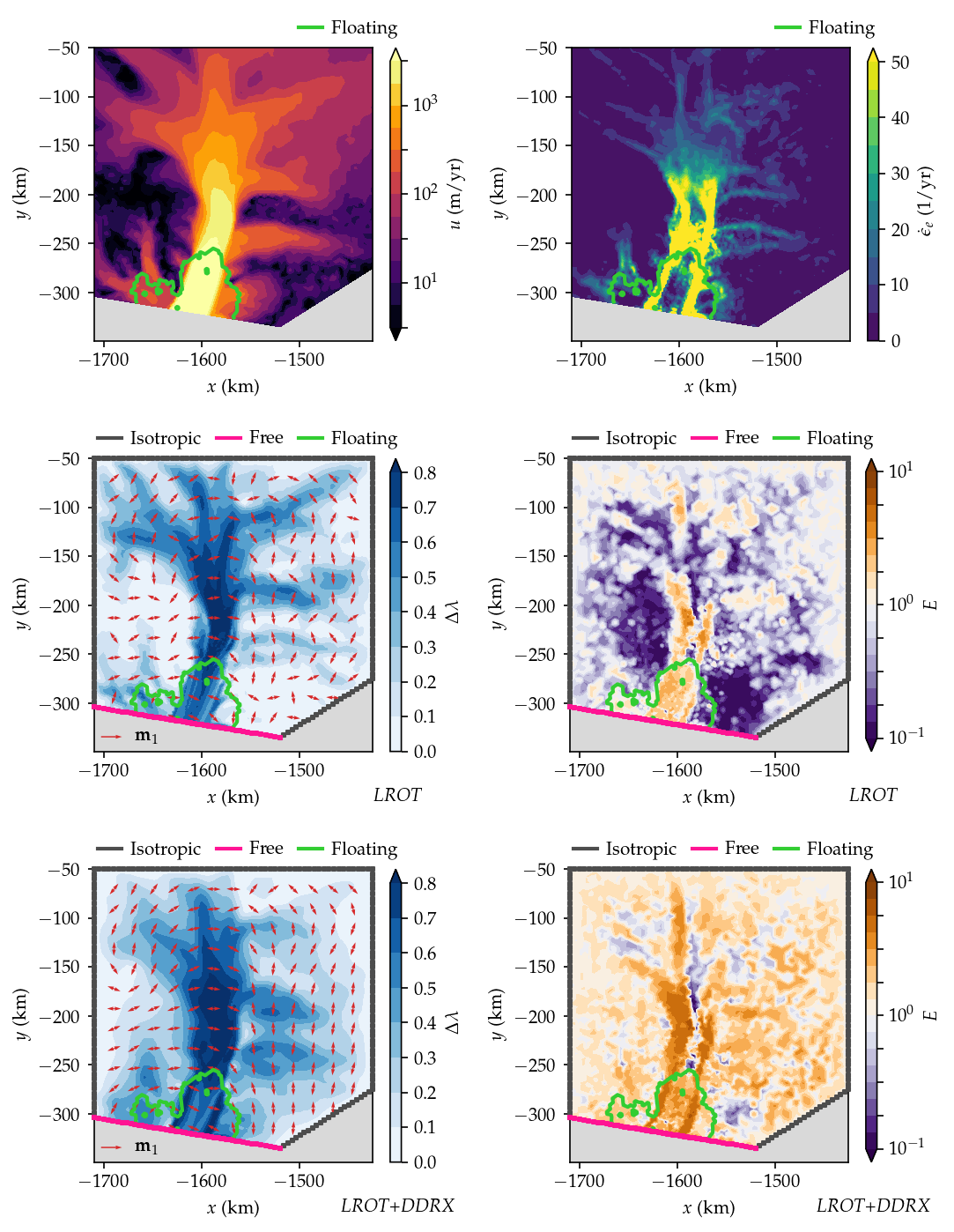
The resulting plots are shown below, where the first row shows the velocity and strain rate field interpolated onto the model mesh, and the second and third row shows model results without and with DDRX, respectively.