Inferring CPO from radar

The dielectric permittivity tensor of a single ice crystal is often taken to be transversely isotropic w.r.t. the crystal \(c\)-axis:

\[ \boldsymbol{\epsilon}' = (2\epsilon_{\perp}' + \epsilon_{\parallel}') \frac{{\bf I}}{3} + (\epsilon_{\parallel}'-\epsilon_{\perp}') \left({\bf c}^2 - \frac{{\bf I}}{3} \right), \]

where \(\epsilon_{\parallel}'\) and \(\epsilon_{\perp}'\) are the components parallel and perpendicular to the \(c\)-axis, respectively, which depend on ice temperature and EM wave frequency (Fujita et al., 2000).

For wave lengths much longer than the average grain size, the bulk permittivity tensor \(\boldsymbol{\epsilon}\) of polycrystalline ice may be approximated as the grain-average permittivity tensor, constructed by averaging \(\boldsymbol{\epsilon}'\) over all grain orientations (over the CPO)

\[ \boldsymbol{\epsilon} \simeq \langle \boldsymbol{\epsilon}' \rangle = (2\epsilon_{\perp}' + \epsilon_{\parallel}') \frac{{\bf I}}{3} + (\epsilon_{\parallel}'-\epsilon_{\perp}') \left(\langle {\bf c}^2 \rangle - \frac{{\bf I}}{3} \right) , \]

where \(\langle {\bf c}^2\rangle\) is the second-order structure tensor, identical to \({\bf a}^{(2)}\).

Thus, because the bulk permittivity tensor \(\boldsymbol{\epsilon}\) can be inferred from EM wave speeds or radar return-power anomalies, so can \(\langle {\bf c}^2 \rangle\).

Radar measurements \(\rightarrow\) CPO

A useful approximation over large parts of ice sheets is that \(\langle {\bf c}^2 \rangle\) has a vertical eigenvector, in which case the Cartesian components are

\[ \langle {\bf c}^2 \rangle = \left[\begin{matrix} a_{xx} & a_{xy} & 0\\ a_{xy} & a_{yy} & 0\\ 0 & 0 & a_{zz} \end{matrix}\right] . \]

Consider then the case where the difference in horizontal eigenvalues of \(\langle {\bf c}^2 \rangle\),

\[ \Delta \lambda = \lambda_2 - \lambda_1, \]

can be inferred from ice-penetrating radar, where \({\bf m}_1\) and \({\bf m}_2\) are the corresponding horizontal eigenvectors and eigenvalues are sorted such that \(\lambda_1 \leq \lambda_2\). It follows that the structure tensor, posed in its eigenframe (\({\bf m}_1, {\bf m}_2, {\bf z}\)), is

\[ \langle {\bf c}^2 \rangle = \left[\begin{matrix} \lambda_1 & 0 & 0 \\ 0 & \lambda_1 + \Delta\lambda & 0 \\ 0 & 0 & 1 - \Delta \lambda - 2\lambda_1 \end{matrix}\right] , \]

where the identity \(\operatorname{tr}(\langle {\bf c}^2 \rangle) = 1\) was used.

Gerber's approximation

Since \(\lambda_1\) is unknown, the problem can be closed by making different assumptions about \(\lambda_1\) given the local/upstream flow regime, such as proposed by Gerber et al. (2023).

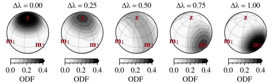
Suppose \(\Delta\lambda\) is measured in region where \(c\)-axes are, to a good approximation, suspected to be distributed on the \({\bf m}_2\)—\({\bf z}\) plane because the smallest eigenvalue is vanishing, \(\lambda_1 \rightarrow 0\). In this case, \(\Delta \lambda = 0\) represents a perfect single-maximum along \({\bf z}\), \(\Delta \lambda = 0.5\) a perfect girdle in the \({\bf m}_2\)—\({\bf z}\) plane, and \(\Delta \lambda = 1\) a perfect single-maximum along \({\bf m}_2\), respectively:

CPO \(\rightarrow\) Enhancement factors

If \(\langle {\bf c}^2 \rangle\) can be inferred from radar measurements following the above method, so can the bulk strain-rate enhancement factors \(E_{ij}\) in the same frame. The enhancements depend, however, also on the fourth-order structure tensor, \(\langle {\bf c}^4 \rangle\), while the bulk permittivity \(\boldsymbol\epsilon\) depends exclusively on \(\langle {\bf c}^2 \rangle\). To overcome this, two approaches can be taken.

Method 1:

Use the IBOF closure of the Elmer/Ice flow model:

import numpy as np
from specfabpy import specfab as sf
lm, nlm_len = sf.init(4) # L=4 is sufficient

### Determine <c^2> from radar-derived Delta lambda
l1 = 0   # lambda_1 = 0 (Gerber's approximation)
dl = 0.5 # Delta lambda = lambda_2 - lambda_1
a2 = np.diag([l1, l1+dl, 1-dl-2*l1]) # structure tensor <c^2> in eigenframe
a4 = sf.a4_IBOF(a2) # Elmer/Ice IBOF closure for <c^4> given <c^2>

Method 2

Use an empirical correlation for determining \(\langle {\bf c}^4 \rangle\) given \(\langle {\bf c}^2 \rangle\) if the CPO is approximately rotationally symmetric.

If the CPO symmetry axis is rotated into the vertical direction, \(\langle {\bf c}^2 \rangle\) depends only on the normalized spectral component \(\hat{n}_2^0 = n_2^0/n_0^0:\)

\[ \langle {\bf c}^2 \rangle = \frac{\bf I}{3} + \frac{2\sqrt{5}}{15} \hat{n}_2^0 \left[\begin{matrix} -1/2 & 0 & 0 \\ 0 & -1/2 & 0 \\ 0 & 0 & 1 \end{matrix}\right] , \]

and \(\langle {\bf c}^4 \rangle\) only on \(\hat{n}_2^0\) and \(\hat{n}_4^0 = n_4^0/n_0^0\) (not shown). The figure below shows the empirical correlation between these two components based on ice-core samples.

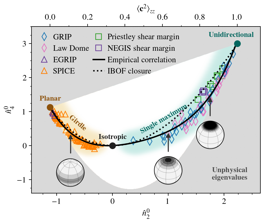
Thus, if \(\hat{n}_2^0\) is extracted from \(\langle {\bf c}^2 \rangle\) in this frame, \(\hat{n}_4^0\) can be derived and hence \(\langle {\bf c}^4 \rangle\) reconstructed. To pose the CPO in the original, unrotated eigenframe (\({\bf m}_1, {\bf m}_2, {\bf z}\)), the resulting expansion series is finally rotated back, allowing eigenenhancements to easily be calculated using specfab.

The following code demonstrates how to take each step with specfab:

import numpy as np
from scipy.spatial.transform import Rotation
from specfabpy import specfab as sf
lm, nlm_len = sf.init(4) # L=4 is sufficient here

### Determine <c^2> from radar-derived Delta lambda
l1 = 0   # lambda_1 = 0 (Gerber's approximation)
dl = 0.5 # Delta lambda = lambda_2 - lambda_1
a2 = np.diag([l1, l1+dl, 1-dl-2*l1]) # second-order structure tensor, <c^2>, in eigenframe
m1, m2, z = np.array([1,0,0]), np.array([0,1,0]), np.array([0,0,1]) # eigenvectors

### Rotate <c^2> into a rotationally-symmetric frame about z
Rm1 = Rotation.from_rotvec(np.pi/2 * m1).as_matrix() # Rotate 90 deg about m1 eigenvector
Rm2 = Rotation.from_rotvec(np.pi/2 * m2).as_matrix() # Rotate 90 deg about m2 eigenvector
if dl < 0.4:         a2_vs = a2 # Already in rotationally-symmetric frame about z
if 0.4 <= dl <= 0.6: a2_vs = np.matmul(Rm2,np.matmul(a2,Rm2.T)) # Rotate vertical (m2--z) girdle into horizontal (m1--m2) girdle
if dl > 0.6:         a2_vs = np.matmul(Rm1,np.matmul(a2,Rm1.T)) # Rotate horizontal (m2) single-maximum into vertical (z) single-maximum

### Determine \hat{n}_4^0 (= n_4^0/n_0^0) from \hat{n}_2^0 (= n_2^0/n_0^0) in rotationally-symmetric frame about z
nhat20 = (a2_vs[2,2]- 1/3)/(2/15*np.sqrt(5)) # azz -> nhat20
nhat40 = sf.nhat40_empcorr_ice(nhat20)[0]

### Construct nlm (state vector) in rotationally-symmetric frame about z
nlm_vs = np.zeros(nlm_len, dtype=np.complex128) 
n00 = 1/np.sqrt(4*np.pi) # only grain-number normalized distribution is known, so must integrate to 1 over S^2.
nlm_vs[0]  = n00
nlm_vs[3]  = nhat20*n00
nlm_vs[10] = nhat40*n00

### Rotate spectral CPO state back to origional (m1,m2,z) eigenframe 
if dl < 0.4:         nlm = nlm_vs # Already in vertical symmetric frame
if 0.4 <= dl <= 0.6: nlm = sf.rotate_nlm(nlm_vs, -np.pi/2, 0) # Rotate horizontal (m1--m2) girdle back into vertical (m2--z) girdle
if dl > 0.6:         nlm = sf.rotate_nlm(sf.rotate_nlm(nlm_vs, -np.pi/2, 0), 0 ,-np.pi/2) # Rotate vertical (z) single-maximum back into horizontal (m2) single-maximum

### Calculate eigenenhancements
# Transversely isotropic monocrystal parameters for ice (Rathmann & Lilien, 2021)
n_grain   = 1        # Power-law exponent: n=1 => linear grain rheology, nonlinear (n>1) is unsupported
Eij_grain = (1, 1e3) # Grain eigenenhancements (Ecc,Eca) for compression along c-axis (Ecc) and for shear parallel to basal plane (Eca)
alpha     = 0.0125   # Taylor--Sachs weight
# Tuple of eigenenhancements (bulk enhancement factors w.r.t. m1, m2, z)
e1, e2, e3 = m1, m2, z
Eij = sf.Eij_tranisotropic(nlm, e1,e2,e3, Eij_grain,alpha,n_grain) # (E_{m1,m1},E_{m2,m2},E_{zz},E_{m2,z),E_{m1,z},E_{m1,m2})
# To calculate bulk enhancement factors w.r.t. other axes of deformation/stress, change (e1,e2,e3) accordingly.

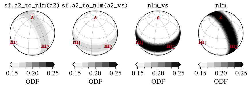
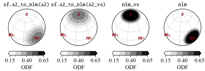
For reference, the following plots show the different CPOs at each step for \(\Delta\lambda=0.5\) and \(\Delta\lambda=1\), respectively: