Strain rate enhancement
Given a bulk anisotropic rheology \({\dot{\boldsymbol\epsilon}}(\boldsymbol\tau)\), where \({\dot{\boldsymbol\epsilon}}\) and \({\boldsymbol\tau}\) are the bulk strain-rate and deviatoric stress tensors, respectively, the directional strain-rate enhancement factors \(E_{ij}\) are defined as the \(({\bf e}_i, {\bf e}_j)\)-components of \({\dot{\boldsymbol\epsilon}}\) relative to that of the rheology in the limit of an isotropic CPO:
for a stress state aligned with \(({\bf e}_i, {\bf e}_j)\):
In this way:
-
\({E_{11}}\) is the longitudinal strain-rate enhancement along \({\bf e}_{1}\) when subject to compression along \({\bf e}_{1}\),
-
\({E_{12}}\) is the \({\bf e}_{1}\)—\({\bf e}_{2}\) shear strain-rate enhancement when subject to shear in the \({\bf e}_{1}\)—\({\bf e}_{2}\) plane,
-
...and so on.
To be clear, \(E_{ij}>1\) implies the material response is softened due to fabric (compared to an isotropic CPO), whereas \(E_{ij}<1\) implies hardening.
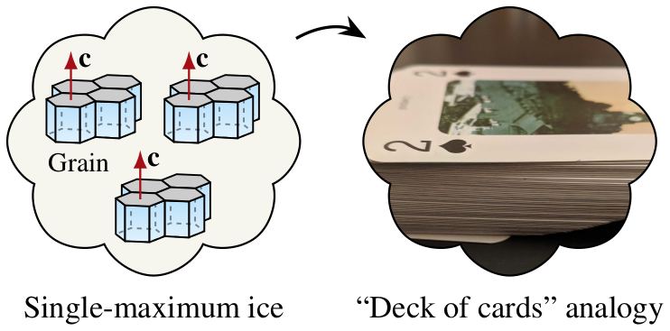
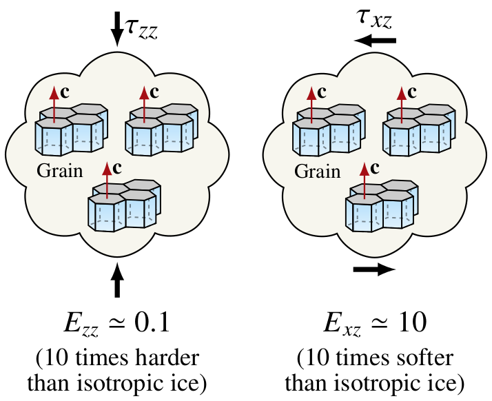
Example: Glacier ice
In the case of glacier ice with a strongly-developed preferred \(c\)-axis direction (single maximum; left figure below), \(E_{ij}\) have been measured in lab tests of compression and shear along the preferred direction (right figure below):
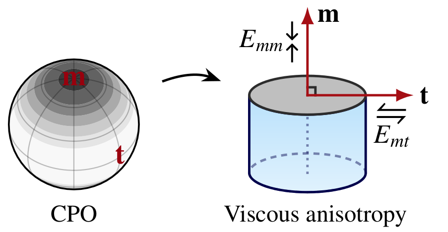
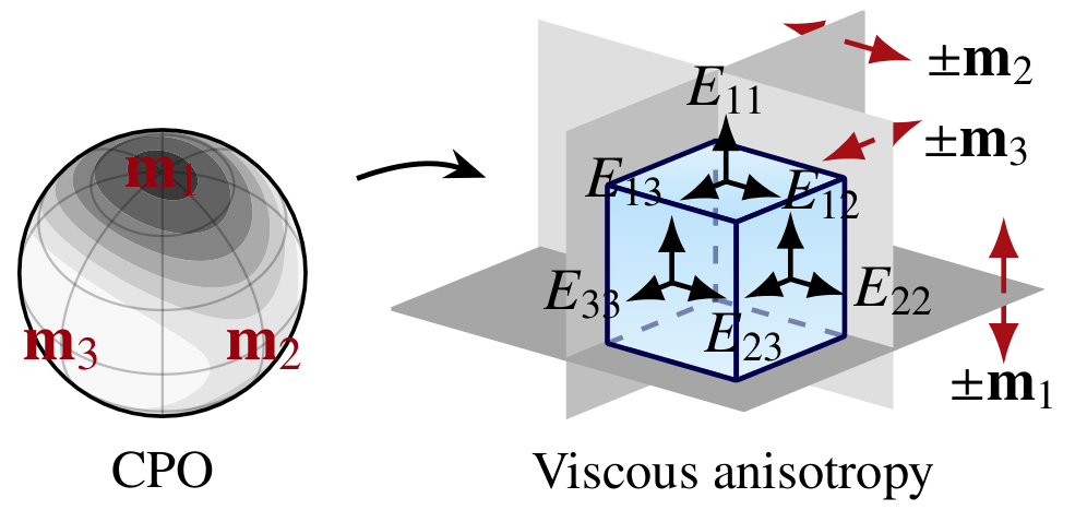
Eigenenhancements
Eigenenhancements are defined as the enhancement factors with respect to the symmetry axes \({\bf m}_i\) of the CPO:
These are the enhancements factors needed to specify the viscous anisotropy in bulk rheologies:
| Transversely isotropic | Orthotropic |
|---|---|
 |
 |
Grain homogenization
Taylor—Sachs
Calculating \(E_{ij}\) using (1) for a given CPO requires an effective rheology that takes the microstructure into account.
In the simplest case, polycrystals may be regarded as an ensemble of interactionless grains (monocrystals), subject to either a homogeneous stress field over the polycrystal scale:
or a homogeneous stain-rate field:
where \({\boldsymbol\tau}'\) and \({\dot{\boldsymbol\epsilon}}'\) are the microscopic (grain-scale) stress and strain-rate tensors, respectively.
The effective rheology can then be approximated as the ensemble-averaged monocrystal rheology for either case:
where \(\langle \cdot \rangle^{-1}\) inverts the tensorial relationship.
If a linear combination of the two homogenizations is considered, equation (1) can be approximated as
or simply
where \(\alpha\in[0;1]\) is a free parameter.
Grain parameters
The grain viscous parameters used for homogenization should be understood as the effective values needed to reproduce deformation experiments on polycrystals; they are not the values derived from experiments on single crystals.
Azuma—Placidi
🚧 Not yet documented.