Deformation kinematics

The deformation gradient tensor \({\bf F}\) quantifies how infinitesimal material elements (line, area, or volume) are deformed relative to some original reference configuration. The strain tensor \({\boldsymbol \epsilon}\) is derived from \({\bf F}\) and is a measure of how a material deforms, excluding rigid body motions like rotation and translation. In continuum mechanics, it is useful to isolate such pure deformation (stretching) from rigid body motion, since the viscous and elastic response of a material when subject external forces is concerned with how easy or hard it is to stretch a material.
Small strain tensor
The symmetric and antisymmetric parts of \({\bf F}\) describe the degree of stretching and the rotation of material elements, respectively, useful for isolating pure deformation (stretching) from rigid body rotations. For small deformations, the strain tensor (formally small strain tensor) is therefore defined as the symmetric part of \({\bf F}\), minus the identity: $$ {\boldsymbol \epsilon} = \frac{1}{2}\left( {\bf F}+{\bf F}^\top \right) - {\bf I}. $$ The strain tensor \({\boldsymbol \epsilon}\) characterizes how a material stretches, compresses, or shears: positive components indicate extension along certain directions, negative components indicate compression, and off-diagonal components correspond to shear deformation.
The antisymmetric part of \({\bf F}\) is related to the component of deformation that describes rigid body rotation (so-called rotation tensor), defined as $$ {\bf w} = \frac{1}{2}\left( {\bf F}-{\bf F}^\top \right) + {\bf I}. $$ Notice that \({\bf F}= {\boldsymbol \epsilon} + {\bf w}\) by definition.
While the strain tensor is the kinematic field of interest for elastic deformation (elastic problems are concerned with displacement), the strain-rate and spin tensors are more relevant for viscous deformation (viscous problems are concerned with velocity, \({\bf u}\)). The strain-rate and spin tensors are simply the rate-of-change of \({\boldsymbol \epsilon}\) and \({\bf w}\), respectively: $$ {\dot{\boldsymbol\epsilon}} = \frac{1}{2}\left(\nabla {\bf u} + \nabla {\bf u}^\top\right) , \quad {\boldsymbol\omega} = \frac{1}{2}\left( \nabla {\bf u} - \nabla {\bf u}^\top \right) , $$ where the velocity gradient tensor is \(\nabla {\bf u} = \dot{{\bf F}} \cdot {\bf F}^{-1}\).
Kinematic modes
Let us now turn to the two common kinematic modes of deformation, pure shear and simple shear, that we will encounter many times throughout this book. Introducing these kinematic modes in terms of their deformation gradient \({\bf F}\) provides a powerful way to describe e.g. how ice deforms below ice divides and domes of ice sheets.

Example of strain tensors

Pure shear
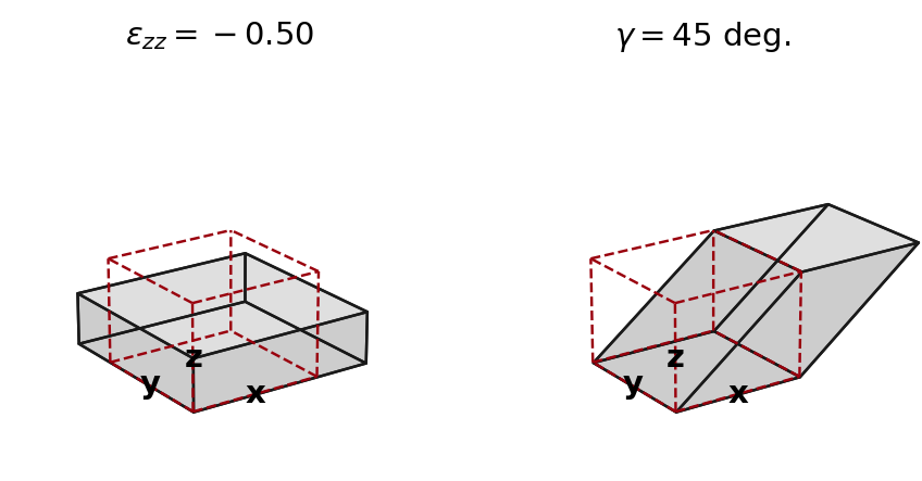
Pure shear (stretching) aligned with the Cartesian coordinate axes renders \({\bf F}\) diagonal, a convenient frame to consider. Suppose shortening takes places along the vertical \(z\)-axis and lengthening in the horizontal \(xy\) plane so that volume is conserved (\(\det({\bf F})=1\); incompressible material). The deformation gradient can then be written as
where \(r\) is a scaling parameter that controls the relative vertical shortening of material lines, and \(q\in[-1;1]\) determines the horizontal direction of lengthening:
- For \(q=0\) lengthening is equal in the \(x\) and \(y\) directions.
- For \(q=+1\) lengthening occurs only in the \(x\) direction.
- For \(q=-1\) lengthening occurs only in the \(y\) direction.
The corresponding vertical strain with time follows immediately as \begin{align} \epsilon_{zz}(t) = r(t) - 1, \end{align} where \(\epsilon_{zz} = 0\) (or \(F_{zz}=1\)) corresponds to the undeformed configuration and \(\epsilon_{zz} = -1\) (or \(F_{zz}=0\)) corresponds to the limit of a vanishing material (parcel) height. Conversely, if lengthening takes place along the vertical axis with shortening in the horizontal plane then \({\bf F}\rightarrow {\bf F}^{-1}\) above, implying \(r\rightarrow r^{-1}\).
Constant strain rate
For pure shear of the above form, it can be shown that the velocity gradient tensor reduces to
Clearly, if \(r\) is written in terms of the \(e\)-folding time \(\tau\),
the strain-rate tensor becomes constant. Specifically, the vertical component becomes
📝 Code example
The above expressions are accessible in specfab as follows
import numpy as np
from specfabpy import specfab as sf
lm, nlm_len = sf.init(4)

axis = 2 # axis of shortening (tauc>0) or lengthening (tauc<0): 0=x, 1=y, 2=z
tauc = 1 # time taken in seconds for parcel to reduce to half (50%) height if tauc>0, or abs(time) taken for parcel to double in height (200%) if tauc<0.
q    = 0 # asymmetry parameter for shortening (if tauc>0) or lengthening (if tauc<0)

tau = tauc/np.log(2)                     # corresponding e-folding time
ugrad = sf.pureshear_ugrad(axis, q, tau) # velocity gradient
D, W = sf.ugrad_to_D_and_W(ugrad)        # strain-rate and spin tensor

t = 1 # some specific time of interest
r   = sf.pureshear_r(tau, t)          # scaling parameter "r" at time t
F   = sf.pureshear_F(axis, q, tau, t) # deformation gradient tensor at time t
eps = sf.F_to_strain(F)               # strain tensor at time t
Simple shear
Simple shear may be characterized by the shear angle \(\gamma\) of the resulting rhombus. In the case of vertical shear in the \(xz\) plane, the deformation gradient tensor is given by
and velocity-gradient tensor becomes
Constant strain rate
For a constant rate of shear \(1/\tau\), where \(\tau\) is a characteristic time, the prefactor is
Solving for the time-dependent shear angle function can be shown to give
Thus, \(\tau\) is the time it takes to reach a shear angle of \(\gamma=45^\circ\) from the undeformed configuration, corresponding to \(\epsilon_{xz}=\tan(45^\circ)/2=0.5\).
📝 Code example
The above expressions are accessible in specfab as follows
import numpy as np
from specfabpy import specfab as sf
lm, nlm_len = sf.init(4)

axis = 2 # axis of shortening (tauc>0) or lengthening (tauc<0): 0=x, 1=y, 2=z
tauc = 1 # time taken in seconds for parcel to reduce to half (50%) height if tauc>0, or abs(time) taken for parcel to double in height (200%) if tauc<0.
q    = 0 # asymmetry parameter for shortening (if tauc>0) or lengthening (if tauc<0)

tau = tauc/np.log(2)                     # corresponding e-folding time
ugrad = sf.pureshear_ugrad(axis, q, tau) # velocity gradient
D, W = sf.ugrad_to_D_and_W(ugrad)        # strain-rate and spin tensor

t = 1 # some specific time of interest
r   = sf.pureshear_r(tau, t)          # scaling parameter "r" at time t
F   = sf.pureshear_F(axis, q, tau, t) # deformation gradient tensor at time t
eps = sf.F_to_strain(F)               # strain tensor at time t
Plotting deformed parcels
Given a deformation gradient \({\bf F}\), the resulting deformed parcel shape can be plotting as follows:
import numpy as np
import matplotlib.pyplot as plt
from specfabpy import specfab as sf
from specfabpy import plotting as sfplt
lm, nlm_len = sf.init(4)

### Determine deformation gradient F

# Pure shear
axis   = 2 # axis of compression/extension (0=x, 1=y, 2=z)
q      = 0 # deformation asymmetry
tau_ps = 1/np.log(2) # e-folding time scale
t_ps   = 1 # time at which deformed parcel is sought
F_ps   = sf.pureshear_F(axis, q, tau_ps, t_ps) # deformation gradient tensor

# Simple shear
plane   = 1 # shear plane (0=yz, 1=xz, 2=xy)
tau_ss  = 1 # characteristic time taken to reach shear strain 45 deg.
t_ss    = 1 # time at which deformed parcel is sought
F_ss    = sf.simpleshear_F(plane, tau_ss, t_ss) # deformation gradient tensor

### Plot
fig = plt.figure(figsize=(6,6))
ax1 = plt.subplot(121, projection='3d')
ax2 = plt.subplot(122, projection='3d')
sfplt.plotparcel(ax1, F_ps, azim=35, axscale=1.7, axislabels=True, drawinit=True)
sfplt.plotparcel(ax2, F_ss, azim=35, axscale=1.7, axislabels=True, drawinit=True)
ax1.set_title(r'$\epsilon_{zz}=%.2f$'%(sf.F_to_strain(F_ps)[2,2]))
ax2.set_title(r'$\gamma=%.0f$ deg.'%(np.rad2deg(sf.simpleshear_gamma(tau_ss, t_ss))))
plt.savefig('deformed-parcel.png', dpi=175, pad_inches=0.1, bbox_inches='tight')