Representation

The Crystallographic Preferred Orientation (CPO) of polycrystalline materials is represented by the distribution of crystal axes in orientation space, $S^2$, weighted by grain size.

Supported grain symmetries, are:

Grain symmetry	CPO components	Definition
Transversely isotropic	$n(\theta,\phi)$	Distribution of slip-plane normals
Orthotropic	$n(\theta,\phi),\,b(\theta,\phi)$	Distribution of slip-plane normals and slip directions

Depending on which crystallographic slip system is preferentially activated, $n(\theta,\phi)$ and $b(\theta,\phi)$ refer to the distributions of different crystallographic axes.

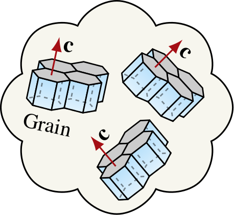
Glacier ice

Polycrystalline ice	Ensemble of slip elements
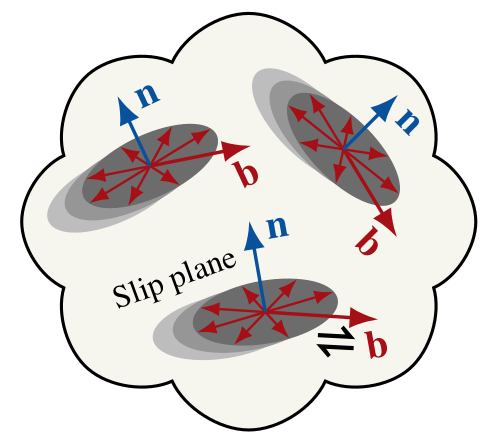		Since ice grains are approximately transversely isotropic, tracking $n(\theta,\phi)$ (the $c$-axis distribution) is sufficient for representing the CPO of glacier ice.

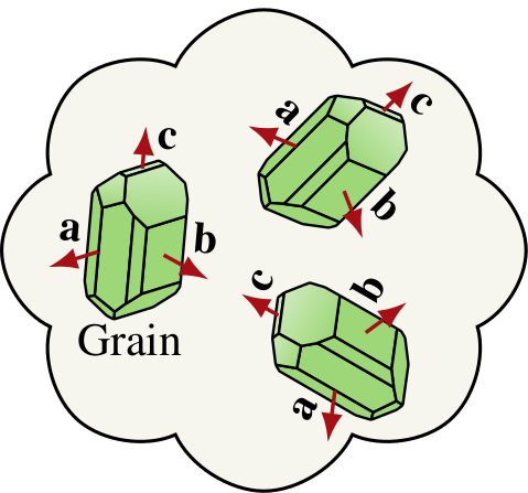
Olivine

Polycrystalline olivine	Ensemble of slip elements
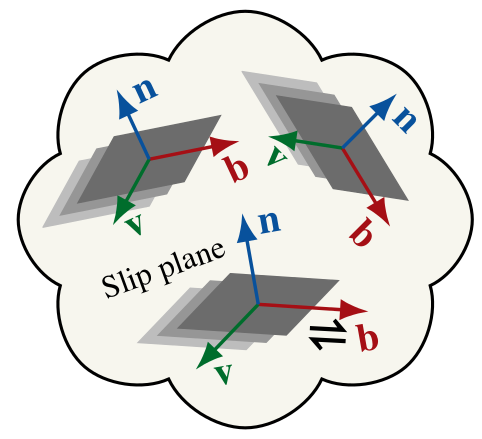		For orthotropic grains such as olivine, both $n(\theta,\phi)$ and $b(\theta,\phi)$ distributions must be tracked to represent the CPO. Notice: $n$ and $b$ represent the distributions of a particular crystallographic axes, depending on fabric type (A—E type).

Background

In specfab, CPOs are defined as the orientation distribution of grains without any reference to grain topology, grain shape, or the spatial arrangement of grains. More precisely, this means statistically describing the directions in which the slip-plane normal and slip direction of grains ($n$- and $b$-axes) are pointing, while also taking into account how massive each grain is (weighted by grain size).

The mass-density orientation distribution function $\rho^{*}({\bf n},{\bf b})$ describes how grain mass is distributed in the space of possible grain orientations (Faria, 2006), where ${\bf n}(\theta,\phi)$ and ${\bf b}(\theta,\phi)$ are arbitrary $n$- and $b$-axes (radial unit vectors). Since $\rho^{*}$ is by definition normalized by the polycrystal volume, integrating $\rho^{*}$ over all possible grain orientations recovers the mass density of the polycrystal (e.g., $\rho=917$ kg/m$^3$ for glacier ice): $$ \rho = \int_{S^2} \int_{S^2} \rho^{*}({\bf n},{\bf b}) \,\mathrm{d}^2{\bf b}\, \mathrm{d}^2{\bf n} , $$ where integration is restricted to the surface of the unit sphere $S^2$ and $\mathrm{d}^2{\bf n}=\sin(\theta)\,\mathrm{d}{\theta}\,\mathrm{d}{\phi}$ is the infinitesimal solid angle in spherical coordinates (similarly for ${\bf b}$).

Ambiguity

Notice that defining the CPO in this way introduces some ambiguity. The contribution to $\rho^{*}({\bf n},{\bf b})$ from two grains with identical mass $m$ and orientation is indistinguishable from a single grain with the same orientation but twice the mass, $2m$. Nonetheless, how well $\rho^{*}({\bf n},{\bf b})$ represents a CPO should ultimately be judged by whether it contains the information necessary to calculate CPO-induced properties to some desired accuracy (say, bulk mechanical anisotropy); not by how simplified it is to disregard the spatial (topological) information of grains.

Glacier ice
In the case of ice, specfab treats for simplicity all monocrystal properties as isotropic in the basal plane (transverse isotropy). This popular approach simplifies the problem significantly: since it does not matter in which direction $b$-axes (crystal $a$-axes) point, there is no need to track how they are distributed. Let therefore $n(\theta,\phi)$ be the corresponding normalized, marginal distribution function of the grain mass-density in the space of possible $n$-axis orientations (crystal $c$-axis orientations): $$ n(\theta,\phi) = \frac{\int_{S^2} \rho^{*}({\bf n},{\bf b})\,\mathrm{d}^2{\bf b}}{\rho} . $$

Olivine
More complicated minerals like olivine are represented by also tracking the marginal distribution of slip directions: $$ b(\theta,\phi) = \frac{\int_{S^2} \rho^{*}({\bf n},{\bf b})\,\mathrm{d}^2{\bf n}}{\rho} . $$ If needed, the joint distribution function $\rho^{*}({\bf n},{\bf b})$ can be estimated from its marginal distributions following the identity for conditional probability density functions and some assumptions.

Mass or number density distributions?

The normalized, marginal distributions $n(\theta,\phi)$ and $b(\theta,\phi)$ are typically referred to as Mass Orientation Distribution Functions (MODFs) or Orientation Mass Distributions (OMDs).

In the literature, number-density distributions, rather than mass-density, frequently appear. In this case, $n(\theta,\phi)/N$ and $b(\theta,\phi)/N$ are referred to as the normalized Orientation Distribution Functions (ODFs) of slip-plane normals and slip directions, respectively, where $N = \int_{S^2} n(\theta,\phi) \,\mathrm{d}^2{\bf n}$ is the total number of grains.

In the models of crystal processes available in specfab, the normalization is conserved and the two views give, in effect, the same result. The mass-density interpretation representation rests, however, on stronger physical grounds, since mass is conserved whereas grain numbers are not.

Harmonic expansion

The distributions $n(\theta,\phi)$ and $b(\theta,\phi)$ are represented as an expansion series in spherical harmonics

\[ n(\theta,\phi)=\sum_{l=0}^{L}\sum_{m=-l}^{l}n_{l}^{m}Y_{l}^{m}(\theta,\phi) \quad\text{(distribution of slip-plane normals)}, \]

\[ b(\theta,\phi)=\sum_{l=0}^{L}\sum_{m=-l}^{l}b_{l}^{m}Y_{l}^{m}(\theta,\phi) \quad\text{(distribution of slip directions)}. \]

The CPO state is therefore described by the state vectors of complex-valued expansion coefficients

\[ {\bf s}_n = [n_0^0,n_2^{-2},n_2^{-1},n_2^{0},n_2^{1},n_2^{2},n_4^{-4},\cdots,n_4^{4},\cdots,n_L^{-L},\cdots,n_L^{L}] \quad\text{($n$ state vector)}, \]

\[ {\bf s}_b = [b_0^0,b_2^{-2},b_2^{-1},b_2^{0},b_2^{1},b_2^{2},b_4^{-4},\cdots,b_4^{4},\cdots,b_L^{-L},\cdots,b_L^{L}] \quad\text{($b$ state vector)}, \]

where the magnitude and complex phase of each coefficient determines the size and rotation that a given harmonic contributes with.

Reduced form

Not all expansion coefficients are independent for real-valued expansion series, but must fulfill

\[ n_l^{-m}=(-1)^m(n_l^m)^* , \]

\[ b_l^{-m}=(-1)^m(b_l^m)^* . \]

This can be taken advantage of for large problems where many (e.g. gridded) CPOs must be stored in memory, thereby reducing the dimensionality of the problem. The vectors of reduced expansion coefficients are defined as

\[ \tilde{{\bf s}}_n = [n_0^0,n_2^{0},n_2^{1},n_2^{2},n_4^{0},\cdots,n_4^{4},\cdots,n_L^{0},\cdots,n_L^{L}] \quad\text{(reduced $n$ state vector)}. \]

\[ \tilde{{\bf s}}_b = [b_0^0,b_2^{0},b_2^{1},b_2^{2},b_4^{0},\cdots,b_4^{4},\cdots,b_L^{0},\cdots,b_L^{L}] \quad\text{(reduced $b$ state vector)}. \]

Converting between full and reduced forms is done as follows (similarly for $\tilde{{\bf s}}_b$):

import numpy as np
from specfabpy import specfabpy as sf
lm, nlm_len = sf.init(6)

### Construct an arbitrary fabric
a2 = np.diag([0.1,0.2,0.7]) # arbitrary second-order structure tensor
nlm = np.zeros((nlm_len), dtype=np.complex64) # array of expansion coefficients
nlm[:sf.L2len] = sf.a2_to_nlm(a2) # l<=2 expansion coefficients from a2
print('original:', nlm)

### Get reduced form of coefficient array, rnlm
rnlm_len = sf.get_rnlm_len() 
rnlm = np.zeros((rnlm_len), dtype=np.complex64) # array of reduced expansion coefficients
rnlm[:] = sf.nlm_to_rnlm(nlm, rnlm_len) # reduced form
print('reduced:', rnlm)

### Recover full form (nlm) from reduced form (rnlm)
nlm[:] = sf.rnlm_to_nlm(rnlm, nlm_len)
print('recovered:', nlm)