Plot CPO

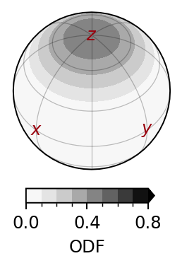
The orientation distribution can be plotted as follows:

import numpy as np
import matplotlib.pyplot as plt
from specfabpy import specfab as sf
from specfabpy import plotting as sfplt
lm, nlm_len = sf.init(6)

### Synthetic CPO to be plotted
a2 = np.diag([0,0,1]) # CPO characterized by a^(2)
nlm = sf.a2_to_nlm(a2) # vector of expansion coefficients

### Setup axes and projection
geo, prj = sfplt.getprojection(rotation=45, inclination=45)
fig = plt.figure(figsize=(2,2))
ax = plt.subplot(111, projection=prj)
ax.set_global() # ensure entire S^2 is shown

### Plot
lvlset = 'iso-up' # default level set: lowest tick/level is the value of an isotropic distribution
lvlset = (np.linspace(0,0.8,9), lambda x,p:'%.1f'%x) # custom level set: (list of levels, how to format colorbar tick labels)
sfplt.plotODF(nlm, lm, ax, cmap='Greys', lvlset=lvlset) # plot distribution (see src/specfabpy/plotting.py for API)
sfplt.plotcoordaxes(ax, geo, color=sfplt.c_dred) # plot coordinate axes (see src/specfabpy/plotting.py for API)
plt.savefig('ODF-plot.png', dpi=175, pad_inches=0.1, bbox_inches='tight')