Matrix model of CPO dynamics

In specfab, CPO evolution is modelled as a matrix problem involving the spectral state vectors of $n(\theta,\phi)$ and $b(\theta,\phi)$.

Mass or number density distributions?

Recall that $n(\theta,\phi)$ and $b(\theta,\phi)$ may equally be understood as the mass density fraction of grains with a given slip-plane normal and slip direction, respectively.

Glacier ice

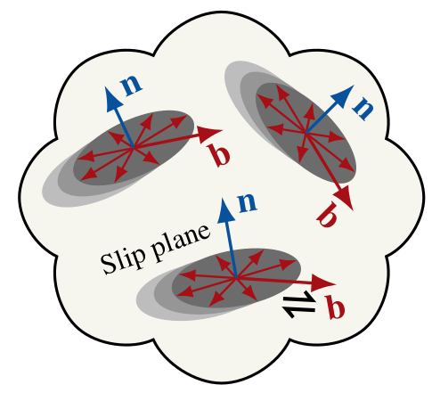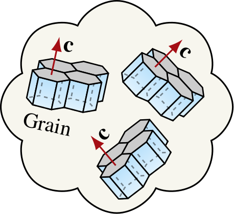
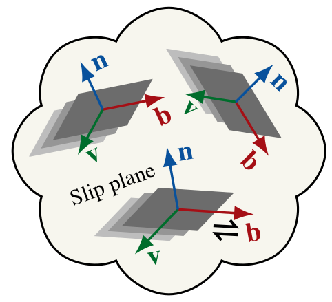
Polycrystalline ice	Ensemble of slip elements

For polycrystalline glacier ice, $n(\theta,\phi)$ is simply the distribution of (easy) slip-plane normals (${\bf n}={\bf c}$). Given the expansion

\[ n({\bf x},t,\theta,\phi)=\sum_{l=0}^{L}\sum_{m=-l}^{l}n_{l}^{m}({\bf x},t) Y_{l}^{m}(\theta,\phi) \quad\text{(distribution of slip-plane normals)}, \]

CPO evolution can be written as a matrix problem involving the state vector

\[ {\bf s} = [n_0^0,n_2^{-2},n_2^{-1},n_2^{0},n_2^{1},n_2^{2},n_4^{-4},\cdots,n_4^{4},\cdots,n_L^{-L},\cdots,n_L^{L}]^{\mathrm{T}} \quad\text{(state vector)}, \]

such that

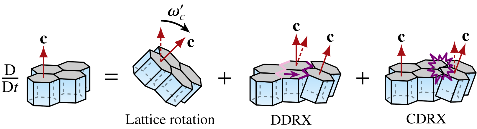
\[ \frac{\mathrm{D}{\bf s}}{\mathrm{D} t} = {\bf M} \cdot {\bf s} \quad\text{(state evolution)}, \]

where the operator (matrix) ${\bf M}$ represents the effect of a given CPO process, which may depend on stress, strain-rate, temperature, etc.

The total effect of multiple processes acting simultaneously is simply

\[ {\bf M} = {\bf M_{\mathrm{LROT}}} + {\bf M_{\mathrm{DDRX}}} + {\bf M_{\mathrm{CDRX}}} + \cdots \quad\text{(operator)}. \]

Validation

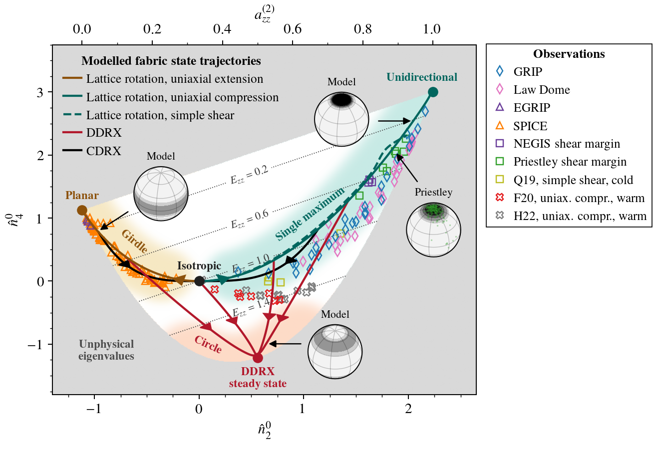
If the CPO is rotated into an approximately rotationally-symmetric frame about the $z$-axis, then only $n_l^0$ components are nonzero. This conveniently allows validating modelled CPO processes by comparing modelled to observed correlations between, e.g., the lowest-order normalized components $\hat{n}_2^0 = n_2^0/n_0^0$ and $\hat{n}_4^0 = n_4^0/n_0^0$. The below plot from Lilien et al. (2023) shows the observed correlation structure (markers) compared to the above CPO model(s) for different modes of deformation, suggesting that modelled CPO processes capture observations reasonably well.

Olivine

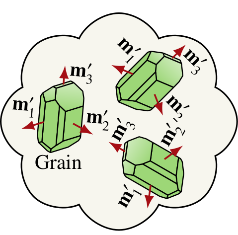
Polycrystalline olivine	Ensemble of slip elements

For polycrystalline olivine, the distributions $n(\theta,\phi)$ and $b(\theta,\phi)$ refer to certain crystallographic axes (${\bf m}'_i$) depending on the fabric type; i.e. thermodynamic conditions, water content, and stress magnitude that control which of the crystallographic slip systems is activated.
Given the expansions

\[ n({\bf x},t,\theta,\phi)=\sum_{l=0}^{L}\sum_{m=-l}^{l}n_{l}^{m}({\bf x},t) Y_{l}^{m}(\theta,\phi) \quad\text{(distribution of slip-plane normals)}, \\ b({\bf x},t,\theta,\phi)=\sum_{l=0}^{L}\sum_{m=-l}^{l}b_{l}^{m}({\bf x},t) Y_{l}^{m}(\theta,\phi) \quad\text{(distribution of slip directions)}, \]

CPO evolution can be written as two independent matrix problems involving the CPO state vector fields

\[ {\bf s}_n = [n_0^0,n_2^{-2},n_2^{-1},n_2^{0},n_2^{1},n_2^{2},n_4^{-4},\cdots,n_4^{4},\cdots,n_L^{-L},\cdots,n_L^{L}]^{\mathrm{T}} \quad\text{($n$ state vector)}, \\ {\bf s}_b = [b_0^0,b_2^{-2},b_2^{-1},b_2^{0},b_2^{1},b_2^{2},b_4^{-4},\cdots,b_4^{4},\cdots,b_L^{-L},\cdots,b_L^{L}]^{\mathrm{T}} \quad\text{($b$ state vector)}, \]

such that

\[ \frac{\mathrm{D}{\bf s}_n}{\mathrm{D} t} = {\bf M}_n \cdot {\bf s}_n \quad\text{($n$ state evolution)}, \\ \frac{\mathrm{D}{\bf s}_b}{\mathrm{D} t} = {\bf M}_b \cdot {\bf s}_b \quad\text{($b$ state evolution)}, \]

where the operators (matrices) ${\bf M}_n$ and ${\bf M}_b$ represents the net effect of CPO processes, similar to the above example for glacier ice.

Supported crystal processes

So far, only lattice rotation is supported for olivine.

Validation

Validation is provided in Rathmann et al. (2024) similar to that above for glacier ice.