CPO dynamics for transversely isotropic grains

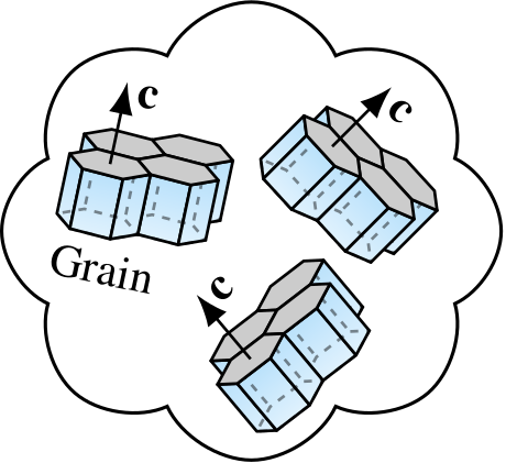
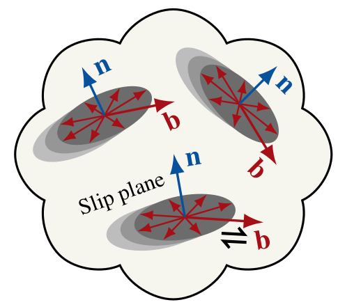
This tutorial focuses on modelling the CPO evolution of polycrystalline glacier ice. That is, the distribution $n(\theta,\phi)$ of (easy) slip-plane normals of grains (${\bf n}={\bf c}$).

Polycrystalline ice	Ensemble of slip elements

Problem

Given the expansion

\[ n({\bf x},t,\theta,\phi)=\sum_{l=0}^{L}\sum_{m=-l}^{l}n_{l}^{m}({\bf x},t) Y_{l}^{m}(\theta,\phi) \quad\text{(distribution of slip-plane normals)}, \]

CPO evolution can be written as a matrix problem involving the state vector

\[ {\bf s} = [n_0^0,n_2^{-2},n_2^{-1},n_2^{0},n_2^{1},n_2^{2},n_4^{-4},\cdots,n_4^{4},\cdots,n_L^{-L},\cdots,n_L^{L}]^{\mathrm{T}} \quad\text{(state vector)}, \]

such that

\[ \frac{\mathrm{D}{\bf s}}{\mathrm{D} t} = {\bf M} \cdot {\bf s} \quad\text{(state evolution)}, \]

where the operator (matrix) ${\bf M}$ represents the effect of a given CPO process, which may depend on stress, strain-rate, temperature, etc.

The total effect of multiple processes acting simultaneously is simply

\[ {\bf M} = {\bf M_{\mathrm{LROT}}} + {\bf M_{\mathrm{DDRX}}} + {\bf M_{\mathrm{CDRX}}} + \cdots \quad\text{(operator)}. \]

Note

$n(\theta,\phi)$ may also be understood as the mass density fraction of grains with a given slip-plane normal orientation. See CPO representation for details.

Lagrangian parcel

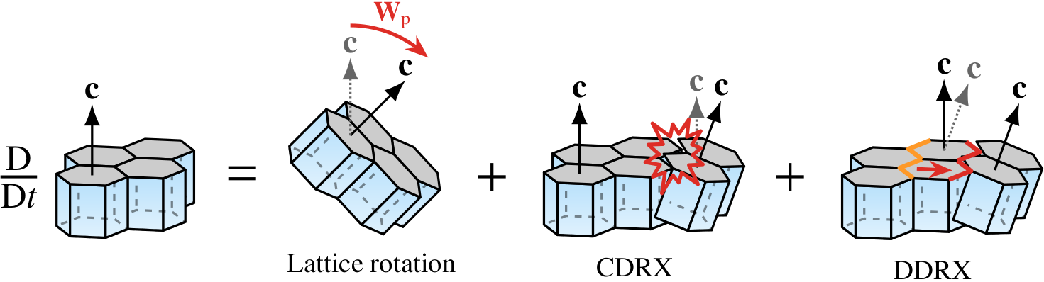
The tutorial shows how to model the CPO evolution of a Lagrangian material parcel subject to three different modes of deformation:

Lattice rotation

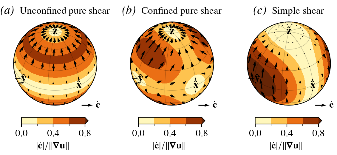
The strain-induced rotation of $c$-axes is modelled given the (local) velocity gradient tensor $\nabla {\bf u}$ (Svendsen and Hutter, 1996). The model is a kinematic model in the sense that $c$-axes rotate in response to the bulk rate of stretching, ${\bf D}$, and spin, ${\bf W}$, thereby allowing the detailed microscopic stress and strain rate fields to be neglected and hence interactions between neighboring grains to be disregarded.

The modelled $c$-axes are taken to rotate with the bulk continuum spin (${\bf W}$), plus some plastic spin correction (${\bf W}_{\mathrm{p}}$), so that the $c$-axis velocity field on the unit sphere is

\[ {\bf \dot{c}} = ({\bf W} + {\bf W}_{\mathrm{p}}) \cdot {\hat {\bf r}} \quad\text{($c$-axis velocity field on $S^2$)} , \]

where ${\hat {\bf r}}$ is the radial unit vector, and the plastic spin depends on ${\bf D}$ to lowest and second lowest order following Wang (1969) and Aravas (1994):

\[ {\bf W}_{\mathrm{p}} = \iota({\hat {\bf r}}\otimes{\hat {\bf r}}\cdot{\bf D} - {\bf D}\cdot{\hat {\bf r}}\otimes{\hat {\bf r}}) + \zeta({\hat {\bf r}}\otimes{\hat {\bf r}}\cdot{\bf D}^2 - {\bf D}^2\cdot{\hat {\bf r}}\otimes{\hat {\bf r}}) . \]

By requiring that basal planes preserve their orientation when subject to simple shear (like a deck of cards), it can be shown that $\iota=1$ and $\zeta=0$.

The corresponding effect on the continuous $c$-axis distribution is modelled as a conservative advection process on the surface of the unit sphere (Fokker—Planck equation on $S^2$):

\[ \frac{\mathrm{D} n}{\mathrm{D} t} = -\nabla_{S^2}\cdot(n{\bf \dot{c}}) \quad\Longrightarrow\quad \frac{\mathrm{D} {\bf s}}{\mathrm{D} t} = {\bf M_{\mathrm{LROT}}} \cdot {\bf s}, \]

where ${\bf M_{\mathrm{LROT}}}$ is given analytically in Rathmann et al. (2021).

c-axis velocity field

The normalized $c$-axis velocity fields for the three modes of deformation considered are:

Example

import numpy as np
from specfabpy import specfab as sf
# L=8 truncation is sufficient in this case, but larger L allows a very strong fabric to develop 
#  and minimizes the effect that regularization has on low wavenumber modes (l=2,4)
lm, nlm_len = sf.init(8) 

### Velocity gradient tensor experienced by parcel
ugrad = np.diag([0.5, 0.5, -1.0]) # Unconfined compression along z-direction (equal extension in x and y)
D = (ugrad+np.transpose(ugrad))/2 # Symmetric part (strain-rate tensor)
W = (ugrad-np.transpose(ugrad))/2 # Anti-symmetric part (spin tensor)

### Numerics 
Nt = 25 # Number of time steps
dt = 0.05 # Time-step size

### Initialize fabric as isotropic
nlm = np.zeros((Nt,nlm_len), dtype=np.complex64) # State vector (array of expansion coefficients)
nlm[0,0] = 1/np.sqrt(4*np.pi) # Normalized ODF at t=0

### Euler integration of lattice rotation + regularization
for tt in np.arange(1,Nt):
    nlm_prev = nlm[tt-1,:] # Previous solution
    iota, zeta = 1, 0 # "Deck of cards" behavior 
    M_LROT = sf.M_LROT(nlm_prev, D, W, iota, zeta) # Lattice rotation operator (nlm_len x nlm_len matrix) 
    M_REG  = sf.M_REG(nlm_prev, D)                 # Regularization operator   (nlm_len x nlm_len matrix)
    M      = M_LROT + M_REG
    nlm[tt,:] = nlm_prev + dt*np.matmul(M, nlm_prev) # Euler step
    nlm[tt,:] = sf.apply_bounds(nlm[tt,:]) # Apply spectral bounds if needed

# See page "Miscellaneous --> Plotting" for how to plot resulting ODFs given nlm

Discontinous dynamic recrystallization (DDRX)

DDRX is modelled as a grain orientation or mass decay/production process on the unit sphere (Placidi and others, 2010):

\[ \frac{\mathrm{D} n}{\mathrm{D} t} = \Gamma n \quad\Longrightarrow\quad \frac{\mathrm{D} {\bf s}}{\mathrm{D} t} = {\bf M_{\mathrm{DDRX}}} \cdot {\bf s} , \]

where the decay/production rate

\[\Gamma = \Gamma_0\left(D- {\langle} D {\rangle}\right) \quad\text{(decay/production rate)}\]

depends on the rate magnitude $\Gamma_0$, and the deformability $D$ as a function of the stress tensor ${\bf S}$:

\[ D = \frac{({\bf S}\cdot{\bf S}):({\hat {\bf r}}\otimes{\hat {\bf r}}) - {\bf S}:({\hat {\bf r}}\otimes{\hat {\bf r}}\otimes{\hat {\bf r}}\otimes{\hat {\bf r}}):{\bf S}}{{\bf S}:{\bf S}}\quad\text{(deformability)} . \]

${\bf M_{\mathrm{DDRX}}}$ is given analytically in Rathmann and Lilien (2021).

Note

The average deformability, $\langle D\rangle$, depends on the instantaneous CPO state — specifically, the structure tensors a2 and a4 — making the corresponding matrix problem nonlinear by conserving the total number of grain orientations or mass density depending on how normalization is interpreted, the latter arguably resting on stronger physical grounds.

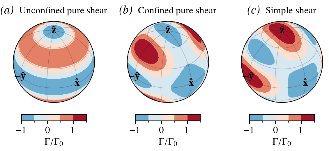
Decay/production rate

The normalized DDRX decay/production rate $\Gamma/\Gamma_0 = D - \langle D \rangle$ is an orientation dependent field that favors nucleation (orientation/mass production) in the directions where the resolved basal-plane shear stress is maximal, and orientation/mass decay elsewhere.

The the normalized decay rate for the three modes of deformation considered are:

Example

import numpy as np
from specfabpy import specfab as sf
# L=8 truncation is sufficient in this case, but larger L allows a very strong fabric to develop 
#  and minimizes the effect that regularization has on low wavenumber modes (l=2,4)
lm, nlm_len = sf.init(8) 

### Stress tensor experienced by parcel
S = np.diag([0.0, 1.0, -1.0]) # Confined compression along z-direction (extension confined to y-direction)
#S = np.diag([0.5, 0.5, -1.0]) # Unconfined compression along z-direction
Gamma0 = 10 # DDRX decay-rate magnitude (may depend on temperature, strain-rate, and other factors, see e.g. Richards et al., 2021)

### Numerics 
Nt = 25 # Number of time steps
dt = 0.05 # Time-step size

### Initialize fabric as isotropic
nlm = np.zeros((Nt,nlm_len), dtype=np.complex64) # State vector (array of expansion coefficients)
nlm[0,0] = 1/np.sqrt(4*np.pi) # Normalized ODF at t=0

### Euler integration of DDRX
for tt in np.arange(1,Nt):
    nlm_prev = nlm[tt-1,:] # Previous solution
    M = Gamma0 * sf.M_DDRX(nlm_prev, S) # DDRX operator (nlm_len x nlm_len matrix)
    nlm[tt,:] = nlm_prev + dt*np.matmul(M, nlm_prev) # Complete Euler step
    nlm[tt,:] = sf.apply_bounds(nlm[tt,:]) # Apply spectral bounds if needed    

# See page "Miscellaneous --> Plotting" for how to plot resulting ODFs given nlm

Continous dynamic recrystallization (CDRX)

Polygonization (rotation recrystallization, CDRX) accounts for the division of grains along internal sub-grain boundaries when exposed to bending stresses. In effect, CDRX reduces the average grain size upon grain division but does not necessarily change the CPO much (Alley, 1992).

The model follows Gödert (2003) by approximating the effect of CDRX on the distribution of grain orientations/mass as a Laplacian diffusive process on $S^2$:

\[ \frac{\mathrm{D} n}{\mathrm{D} t} = \Lambda\nabla^2 n \quad\Longrightarrow\quad \frac{\mathrm{D} {\bf s}}{\mathrm{D} t} = {\bf M_{\mathrm{CDRX}}} \cdot {\bf s} . \]

Example

To model CDRX, add the following contribution to the total fabric operator ${\bf M}$:

M += Lambda*sf.M_CDRX(nlm)

where Lambda is the CDRX rate-factor magnitude, $\Lambda$, that possibly depends on temperature, stress, strain-rate, etc. (Richards et al., 2021).

Regularization

As $n(\theta,\phi)$ becomes anisotropic due to CPO processes, the coefficients $n_l^m$ associated with high wavenumber modes (large $l$ and $m$, and thus small-scale structure) must increase in magnitude relative to the low wavenumber coefficients (small $l$ and $m$).

One way to visualize this is by the angular power spectrum

\[ S(l) = \frac{1}{2l + 1} \sum_{m=-l}^l \left\vert n_l^m \right\vert^2 , \]

which grows with time. In the animation above, the left-hand panel shows how the power spectrum evolves under lattice rotation (unconfined vertical compression) compared to the end-member case of a delta function (dashed line).

If the expansion series is truncated at $l=L$, then $l{\gt}L$ modes cannot evolve, and the truncated solution will reach an unphysical quasi-steady state. To prevent this, regularization must be introduced. Specfab uses Laplacian hyper diffusion ($k>1$) as regularization in $S^2$

\[ \frac{\mathrm{D} n_l^m}{\mathrm{D} t} ={\nu}[l(l+1)]^{k} n_l^m \quad\Longrightarrow\quad \frac{\mathrm{D} {\bf s}}{\mathrm{D} t} = {\bf M_{\mathrm{REG}}} \cdot {\bf s} , \]

that can be added to the fabric evolution operator ${\bf M}$ as follows:

M += sf.M_REG(nlm, D)

This allows the growth of high wavenumber modes to be disproportionately damped (green line compared to red line in animation above).

Note

As a rule-of-thumb, regularization affects the highest and next-highest modes $l{\geq}L-2$ and can therefore not be expected to evolve freely. This, in turn, means that structure tensors a2 and a4, and hence calculated enhancement factors, might be affected by regularization unless $L{\geq}8$ is chosen.

High-level integrator

Alternatively, you can use the high-level Lagrangian parcel integrator for constant stress/strain-rate:

import numpy as np
from specfabpy import specfab as sf
from specfabpy import integrator as sfint
lm, nlm_len = sf.init(8) 

### Process rate factors etc.

iota, zeta = 1, 0       # deck-of-cards behaviour for lattice rotation (=None => disabled)
nu = 1                  # scale the regularization magnitude by this amount (=None => no regularization)
Gamma0 = Lambda = None  # DDRX and CDRX rate factors (=None => disabled)

### Mode of deformation (mod) and parcel strain target 

# Note: axes 0,1,2 = x,y,z, planes 0,1,2 = yz,xz,xy
# See page "Miscellaneous --> Deformation Modes" for T and r definitions
mod, target = dict(type='ps', axis=2, T=+1, r=0), -0.95      # uniaxial compression along z until strain_zz = target
mod, target = dict(type='ps', axis=2, T=-1, r=0), 6          # uniaxial extension along z until strain_zz = target
mod, target = dict(type='ss', plane=1, T=+1), np.deg2rad(80) # simple shear until arctan(strain_xz) = target

### Integrate parcel CPO evolution

nlm0 = np.zeros((nlm_len), dtype=np.complex64)
nlm0[0] = 1/np.sqrt(4*np.pi) # normalized and isotropic initial state
Nt = 200 # Number of integration steps
nlm, F, time, ugrad = sfint.lagrangianparcel(sf, mod, target, Nt=Nt, nlm0=nlm0, iota=iota, zeta=zeta, Gamma0=Gamma0, Lambda=Lambda, nu=nu) # returns (state vector, deformation gradient tensor, time vector, velocity gradient)

# See page "Miscellaneous --> Plotting" for how to plot resulting ODFs given nlm and parcel shape given F

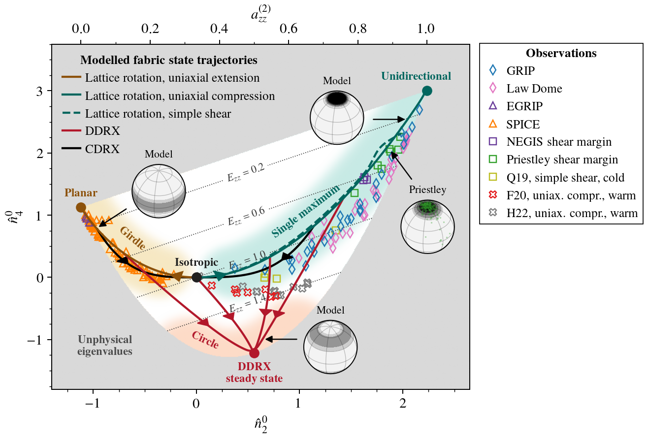
Validation

If the CPO is rotated into an approximately rotationally-symmetric frame about the $z$-axis, then only $n_l^0$ components are nonzero. This conveniently allows validating modelled CPO processes by comparing modelled to observed correlations between, e.g., the lowest-order normalized components $\hat{n}_2^0 = n_2^0/n_0^0$ and $\hat{n}_4^0 = n_4^0/n_0^0$. The below plot from Lilien et al. (2023) shows the observed correlation structure (markers) compared to the above CPO model(s) for different modes of deformation, suggesting that modelled CPO processes capture observations reasonably well.