Viscoplastic constitutive equations

Anisotropic power law rheologies are supported in both forward and inverse (reverse) form. All rheologies assume incompressibility ($\text{tr}({\dot{\boldsymbol\epsilon}})=0$) and are based on classical creep equations where the effective stress $\tau_\mathrm{E}$ has a quadratic form with respect to the invariants $I_i$ of the stress tensor.

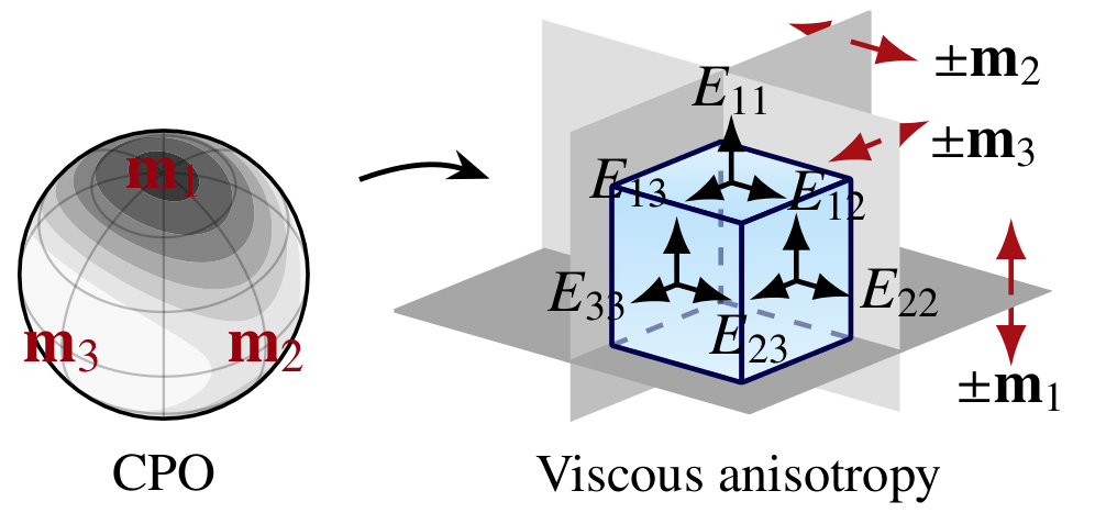
The bulk viscous anisotropy is prescribed in terms of logitudinal and shear strain-rate enhancement factors with respect to the rheological symmetry axes ${\bf m}_i$, termed eigenenhancements $E_{ij}$.

Source of viscous anisotropy

The source of viscous anisotropy is irrelevant for the rheologies that follow. Although specfab is primarily concerned with the effect of CPO development on rheology, the source of viscous anisotropy could equally well be due to aligned cracks, etc.

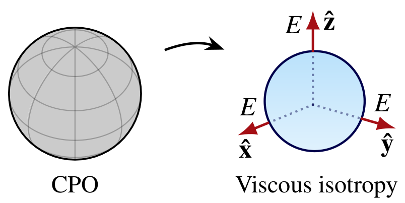
Isotropic

Rheological symmetry	Invariants
	$$ \color{DarkCyan}{I_1 = \mathrm{tr}({\boldsymbol\tau})},\quad I_2 = \mathrm{tr}({\boldsymbol\tau}^2),\quad \color{DarkCyan}{I_3 = \mathrm{tr}({\boldsymbol\tau}^3)}, $$ $\color{DarkCyan}{^*\text{vanish for incompressible, classical creep.}}$

The isotropic rheology is commonly written as

\[ {\dot{\boldsymbol\epsilon}} = A \tau_\mathrm{E}^{n-1} {\boldsymbol\tau} , \\ \tau_\mathrm{E}^2 = I_2 , \hspace{3em} \]

where the flow rate factor $A$ and power law exponent $n$ are free rheological parameters.

Glen flow law

When applied to glacier ice, this rheology is typically referred to as the Glen flow law for isotropic ice. In this case, it is customary to set $\tau_\mathrm{E}^2 = I_2/2$ (divided by 1/2) instead of $\tau_\mathrm{E}^2 = I_2$. If the below anisotropic rheologies are used to model glacier ice, one should therefore set $\tau_\mathrm{E}^2 \rightarrow \tau_\mathrm{E}^2/2$ to ensure that the definition of $A$ is consistent with the Glen flow law.

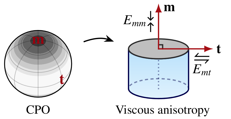
Transversely isotropic

Rheological symmetry	Invariants
	$$ \color{DarkCyan}{I_1 = \mathrm{tr}({\boldsymbol\tau})},\quad I_2 = \mathrm{tr}({\boldsymbol\tau}^2),\quad \color{DarkCyan}{I_3 = \mathrm{tr}({\boldsymbol\tau}^3)},$$ $$ I_4 = {\boldsymbol\tau}:{\bf m}^2, \quad I_5 = ({\boldsymbol\tau}\cdot{\boldsymbol\tau}):{\bf m}^2,$$ $\color{DarkCyan}{^*\text{vanish for incompressible, classical creep.}}$

The transversely isotropic rheology is commonly written as

\[ {\dot{\boldsymbol\epsilon}} = A \tau_\mathrm{E}^{n-1} \Big[ {\boldsymbol\tau} - \lambda_{mm} I_4{\bf I} + \left(3\lambda_{mm}-4\lambda_{mt}\right) I_4{\bf m}^2 + 2\lambda_{mt} ({\boldsymbol\tau}\cdot{\bf m}^2 + {\bf m}^2\cdot{\boldsymbol\tau}) \Big] , \\ \tau_\mathrm{E}^2 = I_2 + \left(3\lambda_{mm}-4\lambda_{mt}\right) I_4^2 + 4\lambda_{mt} I_5 , \hspace{16em} \]

where $A$ is the flow rate factor, $n$ is the power law exponent, and $\lambda_i$ are material parameters. Written in terms of the eigenenhancements, the material parameters are

\[ \lambda_{mm} = \frac{E_{mm}^{2/(n+1)}-1}{2} ,\quad \lambda_{mt} = \frac{E_{mt}^{2/(n+1)}-1}{2} . \]

Alternative form

Unlike the isotropic rheology, the transversely isotropic rheology allows to scale the strain rate components depending on the stress projection along $\bf m$ and in the transverse plane of isotropy. Realizing this, the rheology takes a particularly simple form if rewritten it in terms of the normal- and shear-stress projectors :

\[ {\bf P}_{mm} = {\bf m}^2 - {\bf I}/3, \hspace{7em} \\ {\bf P}_{mt} = \frac{{\boldsymbol\tau}\cdot{\bf m}^2 + {\bf m}^2\cdot{\boldsymbol\tau}}{2} - \boldsymbol\tau:{\bf m}^4 , \]

so that

\[ {\dot{\boldsymbol\epsilon}} = A \tau_\mathrm{E}^{n-1} \Big[ {\boldsymbol\tau} + 3\lambda_{mm} I_{mm} {\bf P}_{mm} + 4\lambda_{mt} {\bf P}_{mt} \Big] , \\ \tau_\mathrm{E}^2 = I_2 + 3\lambda_{mm}I_{mm}^2 + 4\lambda_{mt} I_{mt} , \hspace{6em} \]

where the invariant $I_{mm}$ is equal to the normal stress acting in the plane with the unit normal $\bf m$:

\[ I_{mm} = {\bf P}_{mm} : {\boldsymbol\tau} , \]

and $I_{mt}$ is equal to the square of the shear stress resolved in the transverse plane of isotropy, $\tau^2_\mathrm{RSS}$:

\[ I_{mt} = {\bf P}_{mt} : {\boldsymbol\tau} = ({\boldsymbol\tau}\cdot{\boldsymbol\tau}):{\bf m}^2 - {\boldsymbol\tau}:{\bf m}^4:{\boldsymbol\tau} = \tau^2_\mathrm{RSS} . \]

Free parameters

In addition to $A$ and $n$, the transversely isotropic rheology has three additional rheological parameters that must be specified: $\bf m$, $E_{mm}$, $E_{mt}$.

Special cases

Isotropic limit
In the limit of unit enhancements, $E_{mm},E_{mt}=1$, the isotropic rheology is trivially recovered since $\lambda_{mm},\lambda_{mt}=0$.

Schmid limit
In the case that $E_{mm}=1$ and $E_{mt}\gg 1$, the rheology reduces to the transversely isotropic Schmid rheology that permits only shear deformation in the $\bf m$—$\bf t$ plane.

\[ {\dot{\boldsymbol\epsilon}} = A \tau_\mathrm{E}^{n-1} \left( \frac{{\boldsymbol\tau}\cdot{\bf m}^2 + {\bf m}^2\cdot{\boldsymbol\tau}}{2} - \boldsymbol\tau:{\bf m}^4 \right), \\ \tau_\mathrm{E}^2 = \tau_\mathrm{RSS}^2 \hspace{14em} \]

where a factor of $(4\lambda_{mt})^{(n+1)/2}$ was absorbed into $A$.

API

Forward rheology: D = sf.rheo_fwd_tranisotropic(S, A, n, m, Eij)
Inverse rheology: S = sf.rheo_rev_tranisotropic(D, A, n, m, Eij)

Arguments	Description
`S`, `D`	Deviatoric stress tensor and strain rate tensor (3x3)
`A`, `n`	Flow-rate factor $A$ and power law exponent $n$
`m`	Rotational symmetry axis $\bf{m}$
`Eij`	Tuple of eigenenhancements `(Emm, Emt)`

Orthotropic

Rheological symmetry	Invariants
	$$ ... $$

🚧 Being rewritten, soon available again.