Lagrangian parcel model

Specfab includes a high-level integrator for calculating the CPO evolution of a Lagrangian parcel subject to a constant strain rate tensor. The following code illustrates how to use it, which relies on specifying the kinematic mode of deformation in terms of the DK object.

import numpy as np
from specfabpy import specfab as sf
from specfabpy import integrator as sfint

L = 12 # expansion series truncation
lm, nlm_len = sf.init(L) 

Nt = 200 # number of integration time steps for below mode of deformation (MOD)
nlm = np.zeros((Nt+1,nlm_len), dtype=np.complex64) # expansion coefficients

### Pure shear

axis = 2     # axis of compression (0,1,2 = x,y,z)
tau  = 1     # characteristic e-folding deformation time
q    = +0.25 # asymmetry in directions of extension: q=0 => unconfined, q=+1 or q=-1 => 100% confinement in either of the extending directions
strain_target = -0.95 # deform parcel until this strain target is reached along "axis"

DK = dict(type='ps', q=q, axis=axis, tau=tau) # deformation kinematics

### Simple shear

#plane = 1 # (0,1,2 = yz,xz,xy shear)
#strain_target = np.deg2rad(75) # deform parcel until this target strain (strain angle)
#tau = 1 # characteristic deformation time-scale (1/shearrate)

#DK = dict(type='ss', plane=plane, tau=tau)

### Integrate

kw_dyn = dict(
    iota   = 1,    # plastic spin strength (default: iota=1 for deck-of-cards behaviour)
    nu     = 1,    # multiplicative factor for default regularization strength (default: nu=1)
    Gamma0 = None, # DDRX magnitude (None = disabled)
    Lambda = None, # CDRX magnitude (None = disabled)
)

nlm[:,:], F, time, ugrad = sfint.lagrangianparcel(sf, DK, strain_target, Nt=Nt, **kw_dyn)

"""
Outputs are:
------------
nlm (Nt,nlm_len): Harmonic coefficients at each time step
F (Nt,3,3):       Deformation gradient tensor at each time step
time (Nt):        Total time at each time step 
ugrad (3,3):      Velocity gradient
"""

### Auxiliary

strain_ij = np.array([sf.F_to_strain(F[nn,:,:]) for nn in np.arange(Nt)]) # full strain tensor

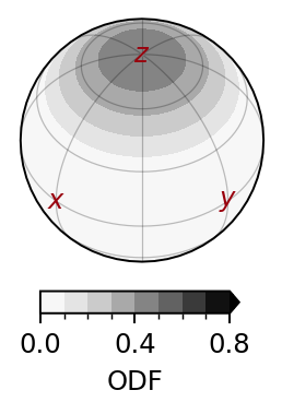
Plot CPO

The orientation distribution (be it ODF or MODF) can be plotted as follows:

import numpy as np
import matplotlib.pyplot as plt
from specfabpy import specfab as sf
from specfabpy import plotting as sfplt
lm, nlm_len = sf.init(6)

### Synthetic CPO to be plotted
a2 = np.diag([0,0,1]) # CPO characterized by a^(2)
nlm = sf.a2_to_nlm(a2) # vector of expansion coefficients

### Setup axes and projection
geo, prj = sfplt.getprojection(rotation=45, inclination=45)
fig = plt.figure(figsize=(2,2))
ax = plt.subplot(111, projection=prj)
ax.set_global() # ensure entire S^2 is shown

### Plot
lvlset = 'iso-up' # default level set: lowest tick/level is the value of an isotropic distribution
lvlset = (np.linspace(0,0.8,9), lambda x,p:'%.1f'%x) # custom level set: (list of levels, how to format colorbar tick labels)
sfplt.plotODF(nlm, lm, ax, cmap='Greys', lvlset=lvlset) # plot distribution (see src/specfabpy/plotting.py for API)
sfplt.plotcoordaxes(ax, geo, color=sfplt.c_dred) # plot coordinate axes (see src/specfabpy/plotting.py for API)
plt.savefig('ODF-plot.png', dpi=175, pad_inches=0.1, bbox_inches='tight')